Section 4.2: The Lorenz equations - detecting chaos

So, where were we? We had found that for certain parameter ranges, the long term behaviour of our system seemed to be unpredictable, and somehow stuck on this strange surface of the Strange Attractor. We’re going to study this system for now in the region just beyond where it becomes truly chaotic, with σ=10, $b=\frac{8}{3}$and $r=25$, just after the Hopf bifurcation.

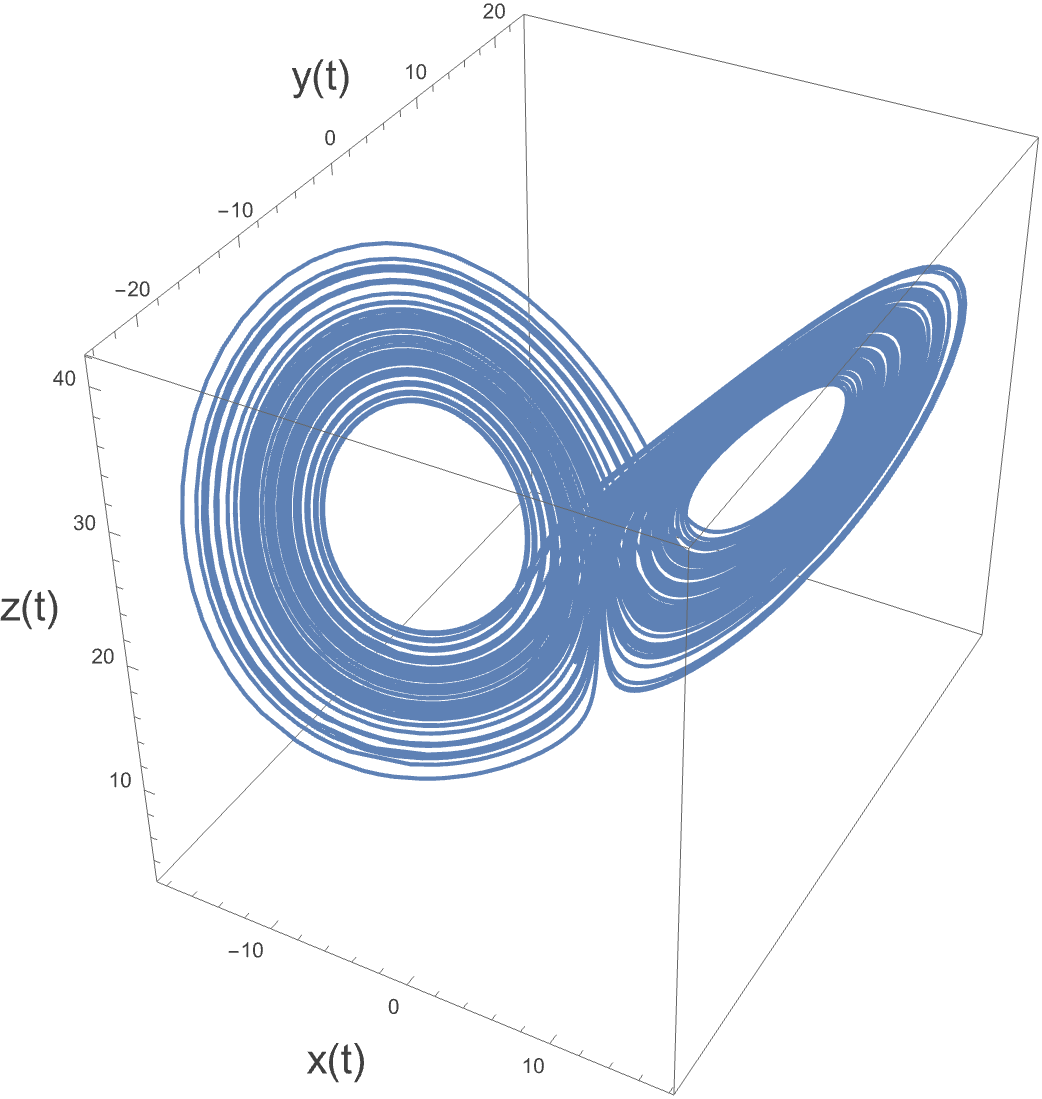
One simple question that we can ask is what happens if you start two trajectories off very close to one another…like really close, and let them play out their trajectories. It’s clear that they can only ever get a finite distance apart, because they will both be stuck on the strange attractor, but really we are interested in the behaviour soon after they set off (so long as they have gone past the transient non-chaotic behaviour).

So we’re going to do the following. We will start a trajectory off from the point $\left(10,-10,0\right)$ and let it run until $t=100$. We will then take that position, and continue running it until $t=200$, along with another trajectory which will start from the same place that the first is at at $t=100$, but shifted in its $x $position by just ${10}^{-15}. $We can then calculate the distance, δ(t), between them as a function of time…however they will start off so close together that we should take

$$ \text{ ln }\left(\delta{}\left(t\right)\right) \text{ where } \delta{}\left(t\right)=|\left(x_{1}\left(t\right),y_{1}\left(t\right),z_{1}\left(t\right)\right)-\left(x_{2}\left(t\right),y_{2}\left(t\right),z_{2}\left(t\right)\right)| $$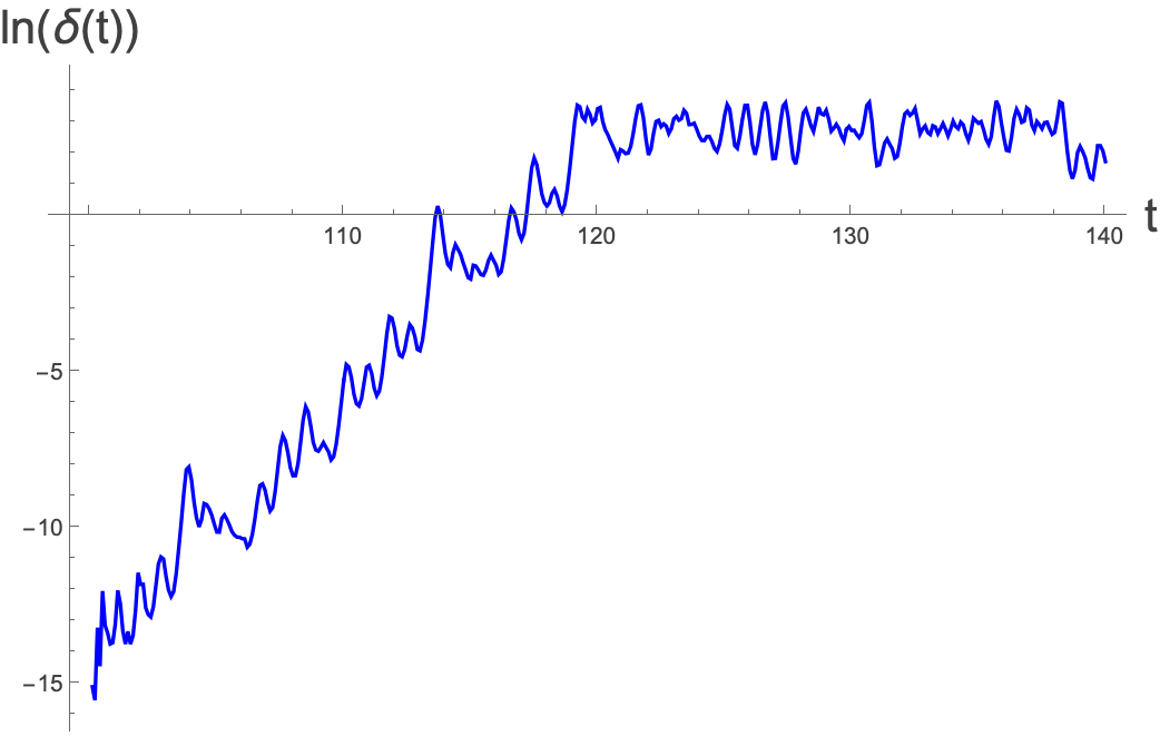

We see here that there are two regimes. One, where we have this rise, and then it seems to level out. It levels out because it’s trapped in a finite region, and they can only get so far apart. What we are interested in is the rise of the first part. If we can calculate the gradient of the first straight line part, then we should have that:

$$ \text{ ln }\left(\delta{}\left(t\right)\right)=a+\lambda{} t \Longrightarrow{}\delta{}\left(t\right)={\delta{}}_{0}e^{\lambda{} t} $$

Note that often δ is defined as the vector quantity, but here I ’m just treating it as the magnitude. Note also that we are taking $t$ here to start at the moment that the second trajectory starts off close to the first.

So let’s do that for the line above:

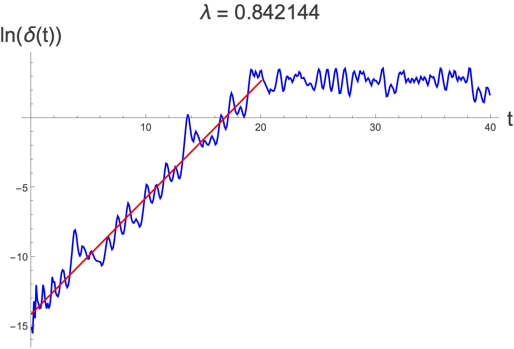
So here we have calculated λ and it gives around 0.84…but that ’s just one particular trajectory. We can do better than this by starting the two trajectories at different times in the first ’s trajectory. Here we take different starting points and create a histogram of the λ we find.

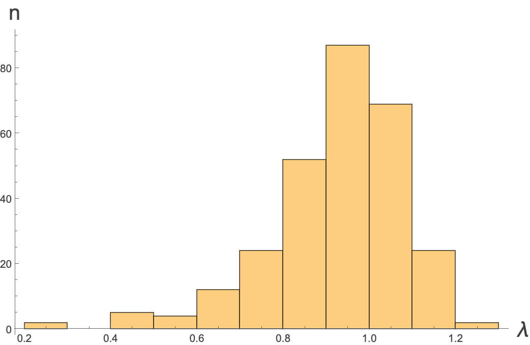
This parameter, λ, which is found numerically is called the Lyapunov exponent - or more accurately a Lyapunov exponent. Rather than asking about two trajectories, starting a little way apart, we can ask about a small sphere of starting points, and ask about how changes its shape changes in different directions.

This exponential behaviour that we have found, with a well-defined Lyapunov exponent is one of the key signs of chaos. We can ask how long into the future out predictions will be good…but it depends on what we mean by good. Let’s say that we want our numerical answer to be within Δ of the true answer. We can ask when

$$ \Delta{}\approx{}{\delta{}}_{0}e^{\lambda{} t_{\text{ horizon }}} \Longrightarrow{} t_{\text{ horizon }}\sim{}O\left(\frac{1}{\lambda{}}\text{ ln }\left(\frac{\Delta{}}{{\delta{}}_{0}}\right)\right) $$

Let’s say then that the precision of our computer is ${10}^{-32}$ - ie. we can set our numbers with up to 32 decimal places of precision. Let’s say that we want our final answer to be within ${10}^{-3} $of the true answer, then

$$ t_{\text{ horizon }}\sim{}O\left(\frac{1}{0.926}\text{ ln }\left(\frac{{10}^{-3}}{{10}^{-32}}\right)\right)=O\left(\frac{1}{0.926}29 \text{ ln }\left(10\right)\right)\sim{}74 $$

So we can project to around 74 units of time into the future here.

Generally if you are doing some simulation then it’s not the precision of the computer which is important, but how good your measurement is. Let’s say that you can only measure the starting conditions up to an accuracy of say ${10}^{-6}$, then we have:

$$ t_{\text{ horizon }}\sim{}O\left(\frac{1}{0.926}\text{ ln }\left(\frac{{10}^{-3}}{{10}^{-6}}\right)\right)=O\left(\frac{1}{0.926}3 \text{ ln }\left(10\right)\right)\sim{}7.7 $$

Not a long time into the future. The thing to note here is that an increase in precision from ${10}^{-6}$ to ${10}^{-32}$ (26 orders of magnitude) only increases the time horizon by a factor of 10.

This exponential behaviour is the first defining property of a chaotic system. The second is that as $t\to \infty{}$ trajectories cannot go to fixed points, and either periodic or quasiperiodic orbits. This shows that the “transient chaos ” that we looked at in the last lesson isn ’t truly chaotic as the long time behaviour actually settled down to one of the fixed points. True chaos can only occur after the Hopf bifurcation where there are no longer any stable fixed points.

The third factor is that our system needs to be deterministic. The seeming unpredictability in the system comes from the non-linear features and not because of any underlying noise in the system. There is a form of chaos called quantum chaos which is not within a deterministic system, but that is something that we will not go into in this course!

The other word that we introduced in the last lecture was this idea of an attractor (be it strange or not). An attractor is some set of points/lines/volume in phase space that has three main properties:

If you start in that set, you remain in that set forever
There is some open set in phase space such that if you start in that set, you will end up in the attractor as $t\to \infty{}$.

There is no proper subset of the attractor that has the above properties.

The Lorenz Map

Let’s just take our prototypical example trajectory above and plot just $z\left(t\right)$:

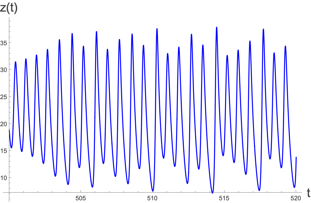
So we are here ignoring the $x \text{ and } y$ directions. We can ask a rather strange question which Lorenz himself asked. Let’s mark the peaks in the above plot. ie. the local maxima in $z:$

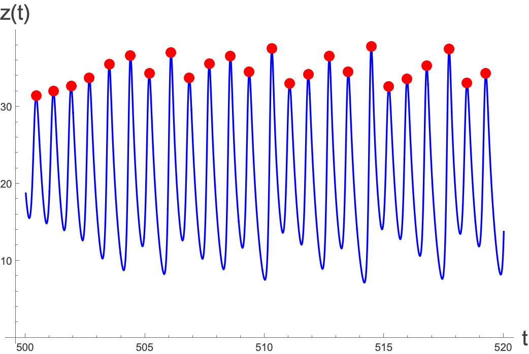
We can label these as $z_{1}$for the position of the first peak, $z_{2}$ for the position of the second peak, etc. Let’s actually put these peaks onto the full trajectory plot to see what we’re doing:

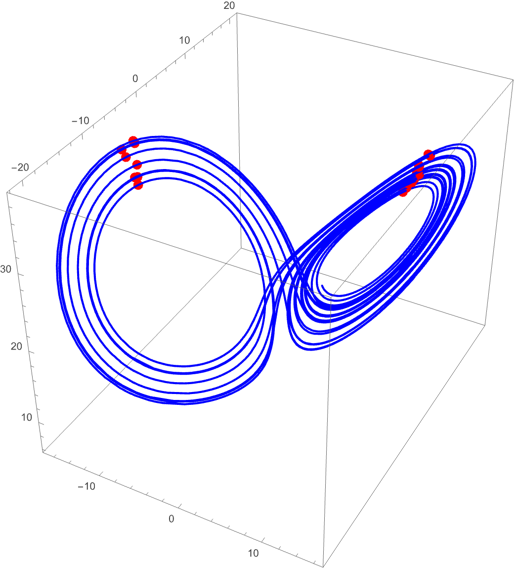
ok, so we’re taking the highest point reached on every pass around the strange attractor. Here we are only plotting for some small time window. Big deal…so what? Well, would you imagine that the $z_{n}$ are related to each other? We can plot $z_{n+1}$ against $z_{n}$ here and we get something rather peculiar. This is a mapping:

$$ Lorenz \text{ mapping }: z_{n}\to z_{n+1} $$

On what follows, the blue dots are values of $\left(z_{n},z_{n+1}\right)$ and the red line is just the line $z_{n+1}=z_{n}$.

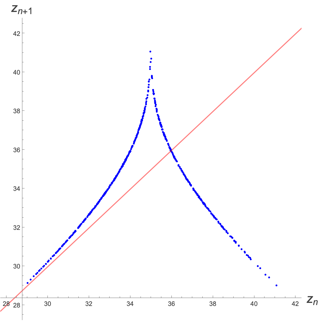
This looks rather like if you were to fill in more and more points it would create a representation of a function $f\left(z\right)$ that would tell you the next $z_{n}$ based on the previous one. Very strangely, this isn’t quite true. The reason that this isn’t true is because for some value of $z_{n}$ there may be more than one $z_{n+1}$. This seems very strange - it essentially says that there are trajectories that have exactly the same maximum height, but are not exactly the same trajectory. If the strange attractor were an infinitely thin surface, this would be true, but it’s not…it’s a criss-crossing mass of trajectories, where they never actually pass through the same point, but they warp over each other in very complex ways. The attractor actually has some sort of thickness, and its dimension can be shown to be a little more than 2…it has a fractal dimension.

OK, so this thing about isn’t quite a perfect curve - it ’s like a curve with some very very fine thickness, but it ’s enough to be able to make predictions using a cobweb diagram (though we have to approximate the points into a curve) to show the path, at least for a fairly reasonable number of ‘returns ’. I’m going to use some code here that I ’ve taken from Sander Huisman: https://community.wolfram.com/groups/-/m/t/153946 and start with $z_{1}=34$.

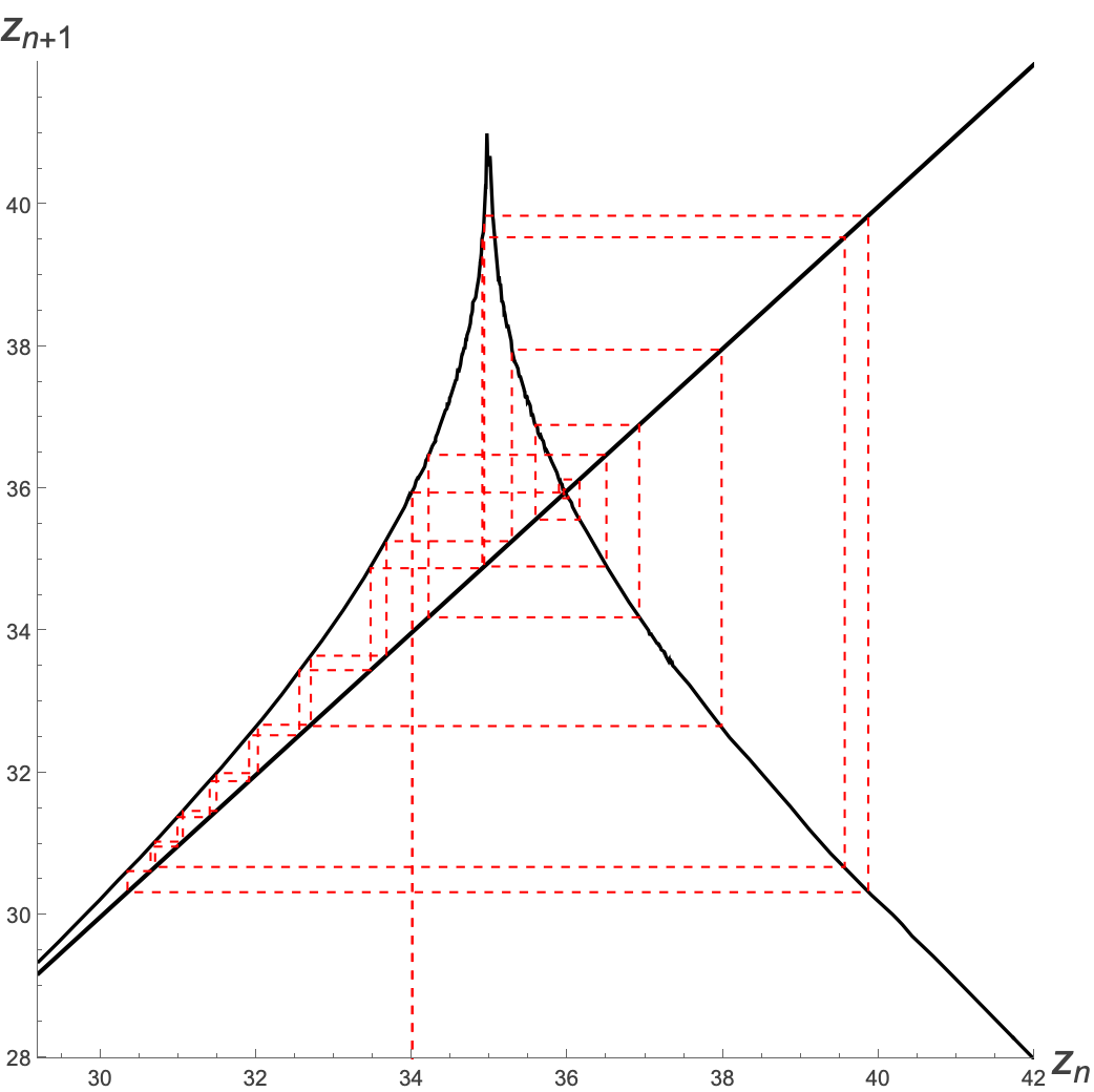
So this looks kind of pretty, but is it useful? Well, strangely, it turns out that it is, and Lorenz used this map to argue for the absence of any stable limit cycles hidden within the Strange Attractor. The question is whether, while we seem to be seeing apparently chaotic behaviour, perhaps there is some very weakly attracting limit cycle that does exist, and trajectories can get attracted to, thus ruling out chaos.

Indeed one thing which is striking, is that there is, seemingly, an intersection between the Lorenz map, and the line $z_{n+1}=z_{n}$. This would mean that there is some value $z^{*}$ for which $f\left(z^{*}\right)=z^{*}$ - ie. a fixed point in the system, and so seemingly some periodic orbit - ie a closed orbit. Can we show that if indeed such a fixed point exists, that it is unstable?

Well, just as in any first order system, to have a fixed point, even in a discrete map, as this is, we can perform a linearisation around the fixed point. We have to be a bit careful though, as what we want to say is that

$$ f\left(z^{*}+{\eta{}}_{n}\right)=z^{*}+{\eta{}}_{n+1} $$

ie. we start off a certain distance ${\eta{}}_{n}$ from the fixed point and we end up a distance ${\eta{}}_{n+1}$from it. Now linearising:

$$ f\left(z^{*}\right)+f'\left(z^{*}\right){\eta{}}_{n}+...=z^{*}+{\eta{}}_{n+1} $$

But because $f\left(z^{*}\right)=z^{*}$ we have the approximation:

$$ f'\left(z^{*}\right){\eta{}}_{n}={\eta{}}_{n+1} $$

Remember that this is a difference equation, and not a differential equation, so there’s going to be no integrating going on here. We do however have:

$$ f'\left(z^{*}\right)=\frac{{\eta{}}_{n+1}}{{\eta{}}_{n}} $$

Taking the absolute value of both sides we have:

$$ |f'\left(z^{*}\right)|=|\frac{{\eta{}}_{n+1}}{{\eta{}}_{n}}| $$

The Lorenz map seems to always have a gradient whose absolute value is greater than 1, in particular at the fixed point:

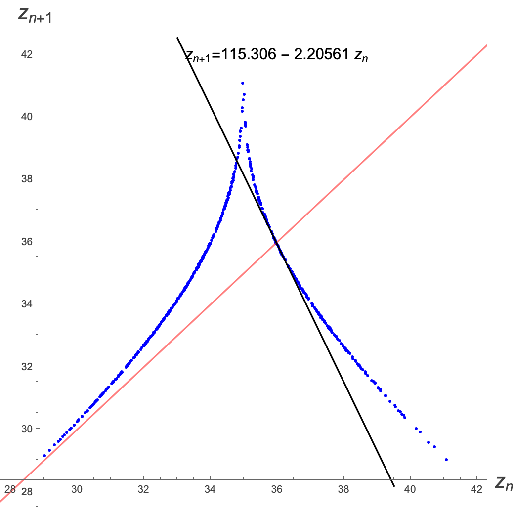
The gradient here has magnitude greater than one, and indeed that is always so . This means that:

$$ |\frac{{\eta{}}_{n+1}}{{\eta{}}_{n}}| >1 $$

Which means that we are moving away from the fixed point. ie. the fixed point is unstable.

But here we have just shown that there isn’t a stable closed orbit that always comes back to the same value of $z_{n}$. Couldn’t there be one that goes between two different values of $z$, or more? Let’s just look at the two period case. This would mean that $z_{n+2}=z_{n}$. We can call this one $z^{*}$, though of course it’s not actually a fixed point.

$$ f\left(f\left(z^{*}\right)\right)=z^{*} $$

But let’s again perturb this:

$$ f\left(f\left(z^{*}+{\eta{}}_{n}\right)\right)=z^{*}+{\eta{}}_{n+2} $$

which we can expand to give:

$$ f\left(f\left(z^{*}\right)+f'\left(z^{*}\right){\eta{}}_{n}\right)\right)=z^{*}+{\eta{}}_{n+2} $$

and then expand the outer $f$ to give:

$$ f\left(f\left(z^{*}\right)\right)+f'\left(f\left(z^{*}\right)\right)f'\left(z^{*}\right){\eta{}}_{n}=z^{*}+{\eta{}}_{n+2} $$

But again we know that $f\left(f\left(z^{*}\right)\right)=z^{*}$:

$$ f'\left(f\left(z^{*}\right)\right)f'\left(z^{*}\right){\eta{}}_{n}={\eta{}}_{n+2} \Longrightarrow{} |f'\left(f\left(z^{*}\right)\right)f'\left(z^{*}\right)|=|\frac{{\eta{}}_{n+2}}{{\eta{}}_{n}}| $$

and the same argument as before holds. All gradients have absolute value greater than 1, so the left hand side is greater than one, and our perturbation has grown. We can do exactly the same thing with any p-cycle, and we will just get a product of derivatives of $f.$ So there can be no stable closed orbits.

So we know that there are no stable fixed points, and we have just argued (if not proved) that there are no stable limit cycles…so it does indeed seem to be chaotic.

One thing which we should be rather careful of here is that we have clearly made a pretty important approximation…and that is that we can talk about the derivative of the Lorenz map…but we said before that it ’s not really a curve, so does it make sense to talk about taking derivatives of it? Well, this is not a formal proof - it is simply an argument based on the observation of the Lorenz map.

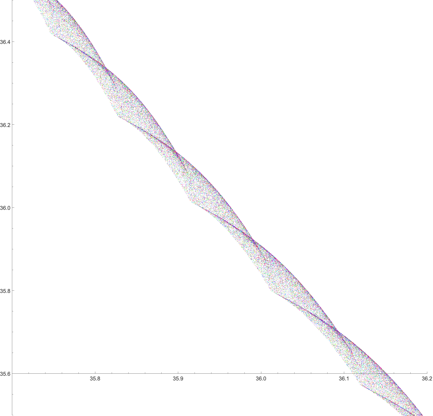
I created the following plot by zooming into one part of the Poincar é map. It looks very pretty, but it turns out that it ’s an artefact of the way I’ve found the values of $z_{\text{ max }}$. This is a warning to heed. Can you see where I made this error?

← Lorenz Equations (Continued)