Section 4.1: The Lorenz equations

Section 4.1: The Lorenz equations

The moment is here…chaos has arrived…finally. Actually, in Greek mythology, chaos was all there was before the creation of the Cosmos, when order came to mess with the natural way of all things…but we ’re getting lost already.

Here we are going to introduce a set of equations which encompass many of the phenomena that we have been speaking about in this course…and more…

We are going to study the famous Lorenz equations:

$$ \dot{x}=\sigma{}\left(y-x\right) $$$$ \dot{y}=r x-y-x z $$$$ \dot{z}=x y-b z $$

where $\sigma{}, r \text{ and } b$ are positive real parameters. These equations look pretty innocuous…they are almost linear, and the non-linearities are just quadratic in the three variables $x, y \text{ and } z$. Ay, there’s the rub…we have three variables, and that is key. We hand-waved our way into believing (correctly), that for non-pathological two-dimensional continuous time systems we can ’t have chaos. But now we have three dimensions, and the cat is well and truly out of the bag and can dart and weave and pirouette in ways that it simply couldn’t in flatland.

These equations came about from a simplified model of how air moves in the atmosphere, but it turns out that this system of equations can be used to describe quite a range of different processes. That’s part of the beauty of mathematical modeling. Often you will find that two systems, when looked at under a slightly blurry microscope, look remarkably similar, and results from one can be ported to the other. In Strogatz he discusses how this system of equations can be used to describe a chaotic waterwheel, and while the example is interesting, I don’t think that it leads to sufficient additional insight that we will use it here. Take a look in his book though for the full exposition.

In fact, the original paper by Lorenz (Lorenz 1963) is surprisingly clear, and you may want to take this as a direction for your review paper project.

Let’s look at the equations and ask about what we might be able to find out about the phase space without solving anything at all (remember…as lazy as possible, but no lazier…). The first equation is linear in $x \text{ and } y$ and is symmetric under $\left(x,y\right)\to \left(-x,-y\right)$. Checking the other equations we see that this symmetry actually holds for all of them. This tells us something about trajectories in the $\left(x,y,z\right) \text{ phase space }$. It says that if there exists some solution $\left(x\left(t\right),y\left(t\right),z\left(t\right)\right)$ for some functions $x, y \text{ and } z, $then there must also be a solution $\left(-x\left(t\right),-y\left(t\right),z\left(t\right)\right)$. This says then that all solutions must either have this as a symmetry, or the solution must have a twin with the $x \text{ and } y$ coordinates replaced by their negatives.

The next property that we can find is that this system is dissipative. This tells us that if we take some region in phase space and evolve it, then over time it will contract. If you know anything about chaos, and the Lorenz equations (and it’s fine if you don’t), this may seem very surprising…but we will see how it reconciles with the ideas of chaos later.

Take some compact region in phase space, inside some closed surface at time $t: $$S\left(t\right)$. Inside this surface is some volume of phase space $V\left(t\right). $After some small amount of time, the points on the surface have all moved, and are making up some new surface $S\left(t+d t\right)$ and of course inside this is a new volume $V\left(t+d t\right).$

Let’s take a one dimensional example. In this case the surface is actually the endpoints of an interval, and the volume is just an interval. Let’s look at the equation:

$$ \dot{x}=x^{2}-1 $$

And let’s ask what happens to the interval $\left[-1.5,-0.5\right]$ under the dynamics of the system. We have that:

$$ \frac{d x}{d t}=x^{2}-1 \Longrightarrow{} d x=\left(x^{2}-1\right) d t $$

So after time $d t$, a point $x \text{ moves to }:$

$$ x+d x=x+\left(x^{2}-1\right) d t $$

and so the interval $\left[-1.5,-0.5\right]$ becomes the interval:

$$ \left[-1.5+\left({\left(-1.5\right)}^{2}-1\right) d t,-0.5+\left({\left(-0.5\right)}^{2}-1\right)d t\right]=\left[-1.5+1.25 d t,-0.5-0.75 d t\right] $$

Which looks like:

So this particular ‘volume’ shrinks in this case. This isn’t surprising because of the fixed point at $x=1$. Note that we have been a bit sloppy with what we’ve done here in taking some finite value for $d t$. Remember that what we have said is really only true in the limit as $d t\to 0$.

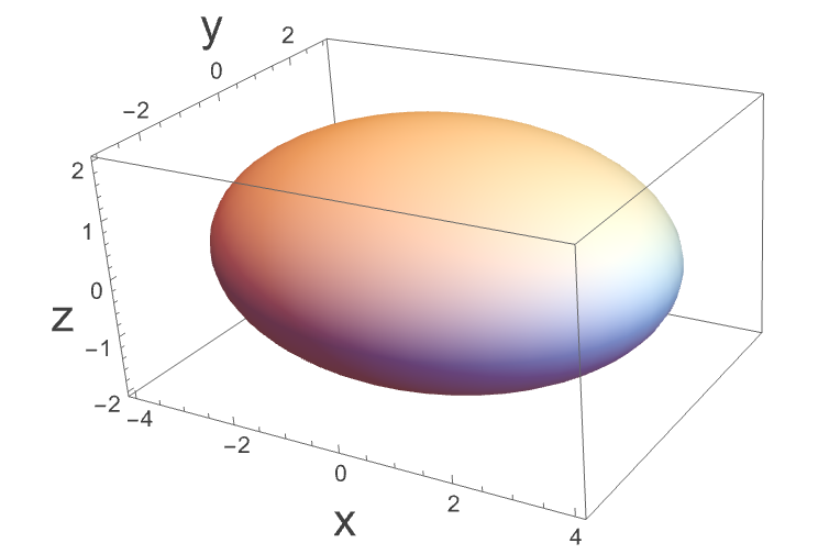
In higher dimensions we need to be more careful because things can shrink and grow in different directions. Let’s say we start off by defining some volume in our phase space as such:

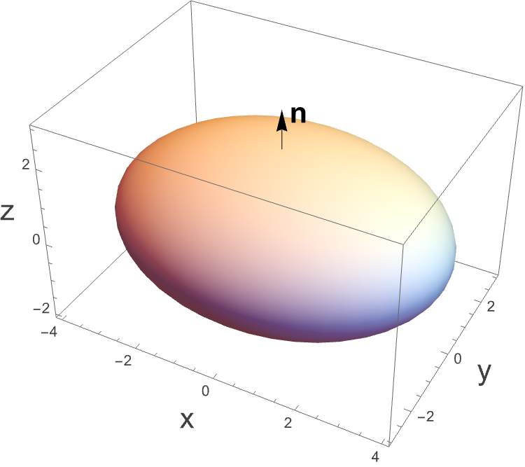
The surface of this shape, $S\left(t\right)$ has, at each point on it a unit normal vector $n$, such as:

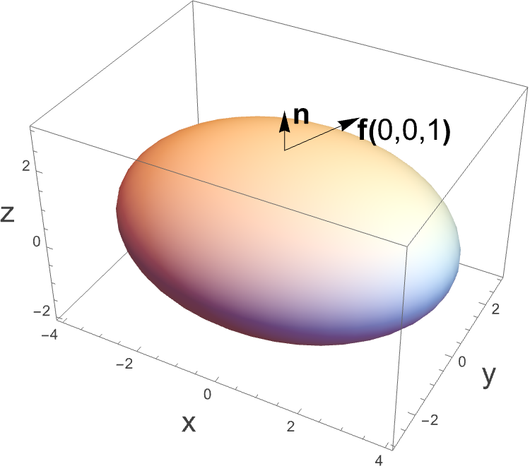
The differential equation of our system can in general be written as a vector field:

$$ \dot{x}=f\left(x\right) $$

which tells us the direction and magnitude of movement of a given point in phase space. In particular, this means that it tells us where points on the sphere move to. $f $defines for us a set of vectors at every point on the surface. Here we just put that vector at one particular point..

What is actually important in terms of the change of volume is only the component of $f$ in the direction of the normal $n$: $n \left(f.n\right)$. We can think about taking some infinitesimal patch of the surface $d A$, which will move some small distance in time $d t$.

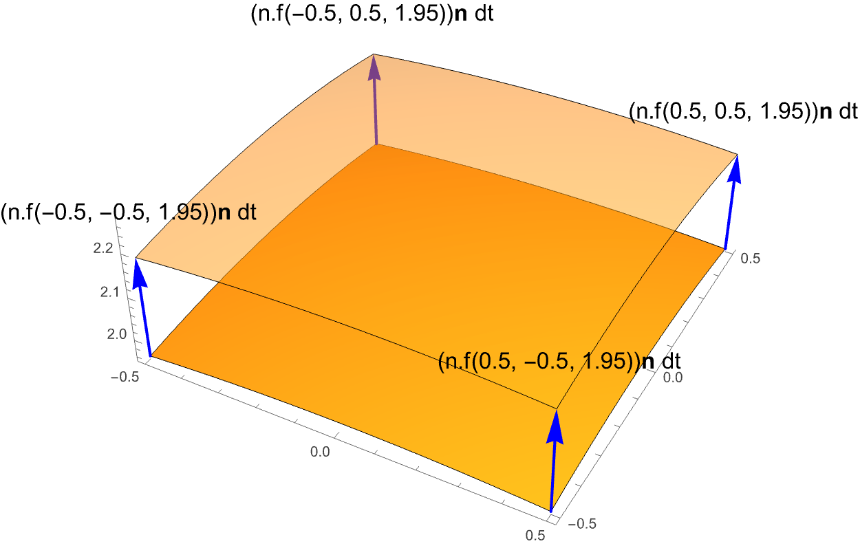
Where the labels correspond to the vectors themselves, not the points at the end of the vectors.

The total volume of this region swept out is:

$$ \left(f.n d t\right)d A $$

And so if we take this and we integrate it over the whole of the surface we get:

$$ V\left(t+d t\right)=V\left(t\right)+{\int{}}_{S\left(t\right)}\left(f.n \text{ dt }\right)\mathrm{d}A $$

and so:

$$ \frac{V\left(t+d t\right)-V\left(t\right)}{\text{ dt }}=\dot{V}={\int{}}_{S\left(t\right)}\left(f.n\right)\mathrm{d}A $$

Then we can use the divergence theorem to get:

$$ \dot{V}={\int{}}_{V}\left(\nabla{}.f\right)\mathrm{d}V $$

where we dropped the $t$ in $V\left(t\right)$ though we know that this is integrated over the volume at time $t $to find the rate of change of the volume at that time.

So for the Lorenz system,

$$ \nabla{}.f={\partial{}}_{x}\left(\sigma{}\left(y-x\right)\right)+{\partial{}}_{y}\left(r x-y-x z\right)+{\partial{}}_{z}\left(x y-b z\right)=-\sigma{}-1-b $$

Which is therefore less than zero. Indeed it is also a constant, so the rate of change in any volume is always negative and is simply proportional to the volume:

$$ \dot{V}=-\left(\sigma{}+1+b\right)V $$

which we can solve to get:

$$ \overset{ }{V}=V_{0}e^{-\left(\sigma{}+1+b\right)t} $$

If you take any volume in phase space, then over time it will shrink exponentially quickly.

Again, doesn’t this sound like exactly the opposite to what you thought chaos was about? Trajectories starting very close together move apart exponentially fast? This sounds like the opposite of that…what is going on?

Well, remember that a volume shrinking does not mean that it shrinks uniformly…this is key!

In fact, we can say something stronger than just that the Lorenz equations tell us that any given volume shrinks over time. We can imagine what happens over a very long time scale which says that if you start with any volume in phase space then

$$ Volume\to 0 \text{ as } t\to \infty{} $$

What?! So everything goes to a point?…not so fast…why just one point? Or indeed why a point at all…what is the volume of a line? What is the volume of a surface? aha…a flash of insight…

Indeed it is true that over time, any volume in phase space in the Lorenz system decreases in volume…but it may be attracted to something more exotic than just a fixed point or a limit cycle…it may be attracted to a so-called Strange Attractor.

We’re going to look at a few more properties of the Lorenz system before exploring the Strange Attractor.

Can the Lorenz system have quasiperiodic solutions? Remember, in a quasiperiodic solution you may have multiple periodic directions and yet overall the system never returns to where it started. In three dimensions, you can have trajectories with at most two periodic directions, which corresponds to the surface of a torus, though it may be some very warped torus. Can we have solutions which are stuck to the surface of a torus in phase space? The surface of the torus can act as the surface to the volume of the torus…and we know that volumes shrink in the Lorenz system, so this is not possible. Hence, there can be no quasiperiodic solutions.

We can also argue, based on this dissipation, that we can’t have any purely repelling fixed points, or repelling closed orbits. Take any point, or orbit that you think is repelling, and put an infinitesimally small volume around it. We know what happens to that volume over time, so it is not possible that all points near to the fixed point/orbit are moving away from it.

Note that this does not preclude saddles. In a saddle there is a repelling direction and an attracting direction, and so we could have a volume which is shrinking, but changing shape such that part of it is expanding (but getting thinner) and another part is contracting.

Indeed we can see that there can only be sinks and saddles, and if there are any closed orbits, they must also be either attractive, or semi-stable.

As usual, we can find the fixed points for this system by setting:

$$ \sigma{}\left(y-x\right)=0 $$$$ r x-y-x z=0 $$$$ x y-b z=0 $$

Solving these gives:

$$ \left(x^{*},y^{*},z^{*}\right)=\left(0,0,0\right), \left(\pm{}\sqrt{b\left(r-1\right)},\pm{}\sqrt{b\left(r-1\right)},r-1\right) $$

Clearly the last two points only exist for $r>1$. They are called $C^{+}$ and $C^{-}$ and appear from the origin at $r=1$. Three fixed points appearing from one sounds a lot like a pitchfork bifurcation, and indeed that’s precisely what happens.

Let’s look at the stability of the fixed points. The Jacobian for the system is our first three dimensional Jacobian:

$$ A=\left(\begin{matrix} -\sigma{} & \sigma{} & 0 \\ r-z & -1 & -x \\ y & x & -b \end{matrix}\right) $$

and thus:

$$ A_{\text{ origin }}=\left(\begin{matrix} -\sigma{} & \sigma{} & 0 \\ r & -1 & 0 \\ 0 & 0 & -b \end{matrix}\right) $$

We see here that the z-direction decouples, and indeed we can see from the equations that close to the origin:

$$ z\left(t\right)=z_{0}e^{-b t} $$

For the $\left(x,y\right)$ plane we have:

$$ \Delta{}=\sigma{}\left(1-r\right), \tau{}=-\left(\sigma{}+1\right) $$

For $r<1$ this is clearly in the $\left(+,-\right) \text{ quadrant }$, so is stable, but we also have that

$$ {\tau{}}^{2}-4\Delta{}={\left(\sigma{}+1\right)}^{2}-4\sigma{}\left(1-r\right)={\left(\sigma{}-1\right)}^{2}+4\sigma{} r>0 $$

so this is a stable node.

For $r<1, $we can actually show that the origin is not only locally stable, but globally so, but using a Lyapunov function

$$ V=x^{2}+\sigma{}\left(y^{2}+z^{2}\right) $$

Remember, this is not a volume, but a quantity (a bit like a potential) which takes on a value at every point in space. We need to show that for all trajectories (for $r<1\right)$ $V \text{ always }$ decreases. We calculate the time derivative, and plug in the equations of motion:

$$ \dot{V}= \dot{x}2x+\sigma{}\left( \dot{y}2y+ \dot{z}2z\right) $$$$ =2\left(x \sigma{}\left(y-x\right)+\sigma{} y \left( r x-y-x z\right)+\sigma{} z \left(x y-b z\right)\right) $$$$ = 2\sigma{}\left( x y-x^{2}+y r x-y^{2}-y x z+z x y-z^{2}b\right) $$$$ = 2\sigma{}\left( x y\left(1+r\right)-x^{2}-y^{2}-z^{2}b\right) $$$$ = 2\sigma{}\left(- {\left(x-\frac{y}{2}\left(1+r\right)\right)}^{2}-y^{2}\left(1-{\left(\frac{1+r}{2}\right)}^{2}\right)-x^{2}-z^{2}b\right) $$

which, so long as $r-1<0$ is necessarily negative. So all trajectories must decrease in their value of $V$…but V is itself like a three dimensional parabola, and so we just roll down it all the way to $\left(0,0,0\right)$ where out V is at a minimum. This proves that the origin is indeed globally stable in this parameter range.

Let’s now look at the system for $r>1$. The origin is now a saddle in the $\left(x,y\right)$ plane and attractive in the $z$ direction. But how about the other fixed points?

The Jacobian at the $C^{\pm{}}$ fixed points is:

$$ A_{C^{\pm{}}}=\left(\begin{matrix} -\sigma{} & \sigma{} & 0 \\ 1 & -1 & \mp{}\sqrt{b\left(r-1\right)} \\ \pm{}\sqrt{b\left(r-1\right)} & \pm{}\sqrt{b\left(r-1\right)} & -b \end{matrix}\right) $$

To understand the nature of these fixed points, let’s solve the eigenvalue system numerically. We have:

$$ \text{ det }\left(\begin{matrix} -\sigma{}-\lambda{} & \sigma{} & 0 \\ 1 & -1-\lambda{} & \mp{}\sqrt{b\left(r-1\right)} \\ \pm{}\sqrt{b\left(r-1\right)} & \pm{}\sqrt{b\left(r-1\right)} & -b-\lambda{} \end{matrix}\right)=0 $$

which gives:

$$ -\left(\sigma{}+\lambda{}\right)\left(\left(1+\lambda{}\right)\left(b+\lambda{}\right)+b\left(r-1\right)\right)-\sigma{}\left(\left(-\left(b+\lambda{}\right)\right)+b\left(r-1\right)\right)=0 $$

Expanding this out, we have:

$$ {\lambda{}}^{3}+{\lambda{}}^{2} \left(1+b+\sigma{}\right)+\lambda{} \left(b\left(r+\sigma{}\right)\right)+2b \sigma{}\left(r -1\right)=0 $$

We can ask what happens for $r=1$ and we have:

$$ {\lambda{}}^{3}+{\lambda{}}^{2} \left(1+b+\sigma{}\right)+\lambda{} \left(b\left(1+\sigma{}\right)\right)=0 $$

Which gives:

$$ \lambda{}=0, \lambda{}=-b, \lambda{}=-1-\sigma{} $$

So at least at this point the eigenvalues are all real. In fact if we increase $r $a little, they remain real, until…well, at

ok, so this is pretty ugly! But you can figure out when you go from a stable node to a stable spiral-type solution by plugging in values for σ and $b$.

Fixing $\sigma{}=10 \text{ and } b=\frac{8}{3}$ (values which are often used), we can numerically calculate the positions of the three roots as a function of $r$. The red line here just traces the history of the eigenvalues.

We see that we start off at the pitchfork bifurcation point (at $r=1\right)$ with all three eigenvalues being real and negative, or zero, corresponding to a stable node. As we increase $r$ we get one real negative eigenvalue and two complex ones (with negative real parts). This corresponds to having a stable direction, and a stable spiral plane.

We then see that at some value of $r$ the sign of the real part of two of the eigenvalues goes from negative to positive, meaning that we now have a stable direction (the negative real eigenvalue) and an unstable spiral plane. The nature of the fixed points has changed, and this can happen via an unstable limit cycle enclosing the previously stable fixed point. This is a Hopf bifurcation and we denote the value of $r $that it happens at as $r_{H}$. Can we calculate this point analytically? Indeed we can. At the Hopf bifurcation point, we know that we have a purely imaginary eigenvalue (and its conjugate):

Remember, our eigenvalue equation is:

$$ {\lambda{}}^{3}+{\lambda{}}^{2} \left(1+b+\sigma{}\right)+\lambda{} \left(b\left(r+\sigma{}\right)\right)+2b \sigma{}\left(r -1\right)=0 $$

Making an ansatz that we have a purely imaginary eigenvalue is equivalent to saying that

$$ \lambda{}=i \omega{} $$

For some real ω.

Substituting this we get:

$$ -i {\omega{}}^{3}-{\omega{}}^{2} \left(1+b+\sigma{}\right)+i \omega{} \left(b\left(r+\sigma{}\right)\right)+2b \sigma{}\left(r -1\right)=0 $$

This is a nice trick because we can separate out the real and imaginary parts:

$$

• {\omega{}}^{3}+ \omega{} \left(b\left(r+\sigma{}\right)\right)=0 $$

$$ -{\omega{}}^{2} \left(1+b+\sigma{}\right)+2b \sigma{}\left(r -1\right)=0 $$

These can be solved separately to give, for the first:

$$ \omega{}=0, \pm{}\sqrt{b\left(r+\sigma{}\right)} $$

and for the second:

$$ \omega{}=\pm{}\sqrt{\frac{2b \sigma{}\left(r-1\right)}{1+b+\sigma{}}} $$

These of course have to be the same ω. For positive $b \text{ and } \sigma{}$ and $r>1$, the second set of solutions cannot be 0, so we can discard that solution. For the other, we can equate the ω:

$$ \sqrt{b\left(r+\sigma{}\right)}=\sqrt{\frac{2b \sigma{}\left(r-1\right)}{1+b+\sigma{}}} $$

Solving for $r \text{ we have }$:

$$ r_{H} =\sigma{}\frac{\left(3+b +\sigma{}\right)}{\left(\sigma{}-b-1\right)} $$

So now we have that for:

$$ 1we have linear stability. Note that this also requires that $\sigma{}>b+1$ otherwise the denominator is negative and we can’t have negative $r.$

Let’s just look at the other eigenvalue at this point. We must have that

$$ {\lambda{}}^{3}+{\lambda{}}^{2} \left(1+b+\sigma{}\right)+\lambda{} \left(b\left(r+\sigma{}\right)\right)+2b \sigma{}\left(r -1\right)=\left(\lambda{}-{\lambda{}}_{1}\right)\left(\lambda{}-{\lambda{}}_{2}\right)\left(\lambda{}-{\lambda{}}_{3}\right) $$

We have found two of the eigenvalues:

$$ \lambda{}=\pm{}i\sqrt{b\left(r+\sigma{}\right)} $$

So substituting this in, we get:

$$ {\lambda{}}^{3}+{\lambda{}}^{2} \left(1+b+\sigma{}\right)+\lambda{} \left(b\left(r+\sigma{}\right)\right)+2b \sigma{}\left(r -1\right)=\left(\lambda{}-i\sqrt{b\left(r+\sigma{}\right)}\right)\left(\lambda{}+i\sqrt{b\left(r+\sigma{}\right)}\right)\left(\lambda{}-{\lambda{}}_{3}\right) $$

Expanding out in λ and solving for ${\lambda{}}_{3}$ we have:

$$ {\lambda{}}_{3}=-\left(\sigma{}+b+1\right) $$

Let’s just look at our bifurcation diagram (in the $\left(r,x\right) \text{ plane }$), again for $b=\frac{8}{3},\sigma{}=10$:

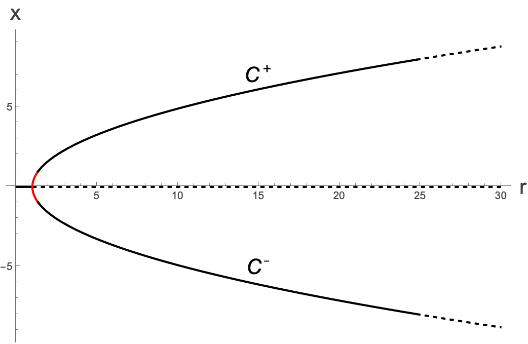
Here the red line denotes where the two fixed points go from being stable nodes to stable spirals.

So we have our pitchfork bifurcation at $r=1,$ and then our Hopf bifurcation at $r_{H}$…but we should really include the limit cycle positions on the above graph. But what does it mean to take an $x$ position of a limit cycle? A limit cycle is a one dimensional ring in the three dimensional space, and so really we should be plotting the positions of the fixed points, and the limit cycles in the full phase plane and see what happens as $r$ changes.

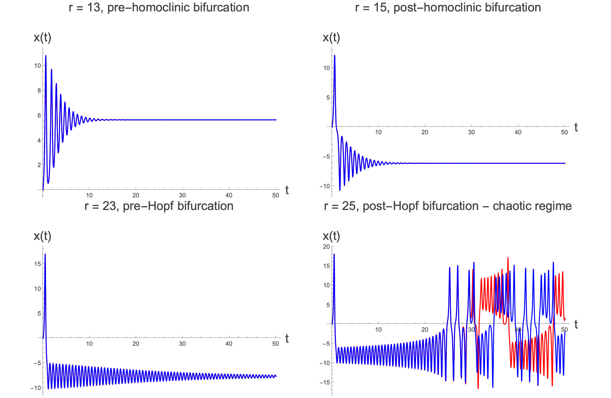
It’s actually not easy to plot the limit cycles, but what we can do is to get an idea of where the homoclinic bifurcation is. We do this by looking at trajectories that start near the origin, and increasing r. You will see that they spiral into the two new fixed points, but at some point the spirals seem to somehow hit the origin. This is a pair of homoclinic orbits and corresponds to the homoclinic bifurcation where the limit cycles first appear. It happens at around $r=14$. In the animation you’ll see that we slow things down around $r=14$ and we’re going to stop just before $r=r_{H} $because we don’t want to spoil the surprise.

Note that at the point of the homoclinic bifurcation, we seem to swap which fixed point each of the trajectories is being attracted to.

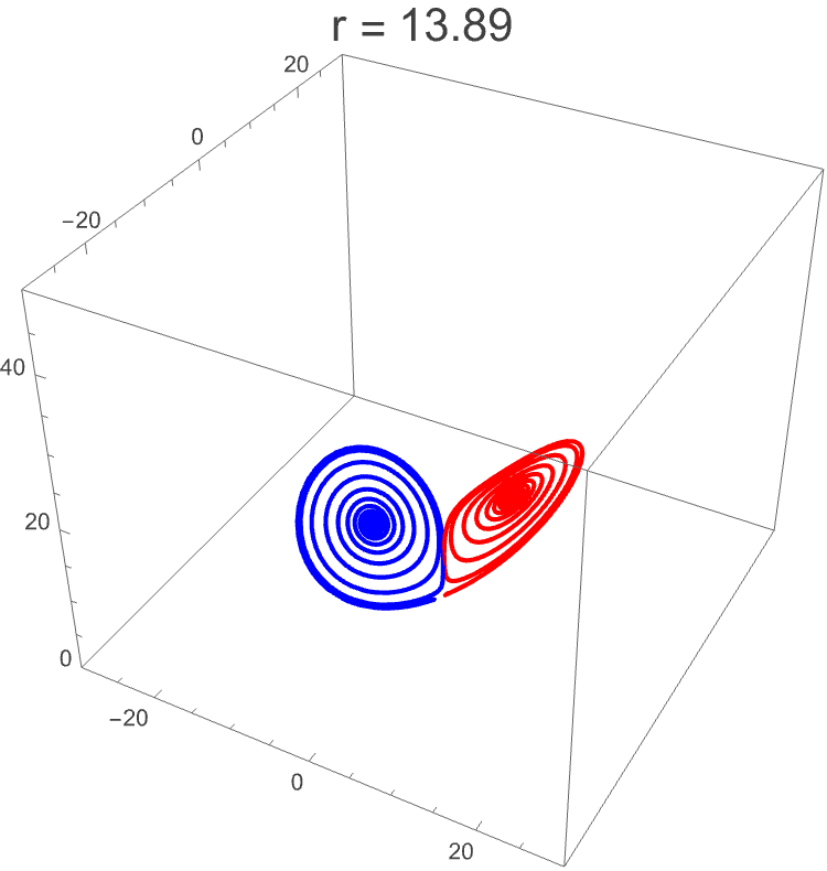
So here we have seen the homoclinic bifurcation via the coming together of the two spirals. At this point, two unstable limit cycles are produced. To plot the positions of the unstable limit cycles is not easy, but I was very lucky to get help from Christopher Klausmeier who has produced an incredible package to study dynamical systems with called EcoEvo. It can be found here: http://raw.githubusercontent.com/cklausme). His website is also worth taking a look at: https://www.kl-lab.group if you want to see where some of the techniques that we have been talking about through this course are applied. Anyway, here we see the unstable limit cycles appear at the point of the homoclinic bifurcation, and then collapse in on the stable fixed points. The largest limit cycles are for $r=14.1$ and the smallest are for $r=24.6$. I have included the code to generate these figures in a separate notebook here.

As $r$ increases, the unstable limit cycle collapses in on the stable fixed points and the fixed points become unstable. We can also plot the positions of these unstable limit cycles by projecting each one’s largest $x$ position:

This picture at $r=13.89$ is the point of the homoclinic bifurcation where the unstable limit cycles comes into existence.

Note here that we are discussing limit cycles in three dimensions all of a sudden. Should our intuition for them from two dimensions hold? Well, a closed orbit is still just a closed orbit in three dimensions, even though it might not stick to some flat plane in three dimensions, and the definition of a limit cycle that we had in two dimensions carries over to three. So the idea of a limit cycle closing in on a fixed point still holds, to give us a supercritical Hopf bifurcation in three dimensions.

What is a bit different is that we have a new type of limit cycle in three dimensions called a saddle cycle where there may be a stable limit cycle in a plane, as well as an unstable direction, or vice versa.

In this case we have an unstable limit cycle, and a stable direction. It ’s like a cross between a saddle and an unstable limit cycle and is actually a little unintuitive, but is important for understanding what ’s happening in the system as we go towards the chaotic regime, though we are not there yet.

In Strogatz an analogue of the following picture is presented

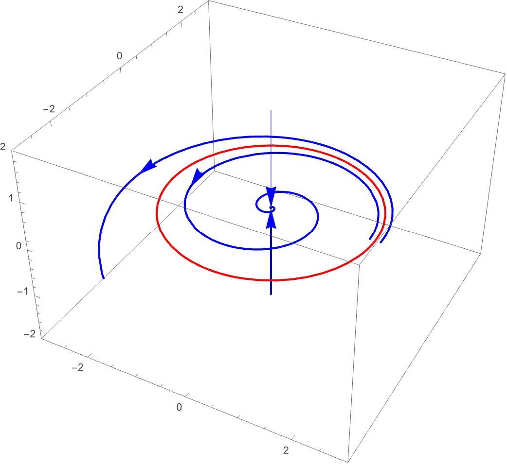
Where there is a plane with an unstable limit cycle (in red) and then a perpendicular stable direction. This is a partial picture, but it doesn ’t quite give an intuition about what happens off the plane. The limit cycle only exists in the plane itself (and in the Lorenz case the plane isn’t even flat), and so we have this sort of tube above and below of regions which will be attracted to the fixed point…but what happens to flows which start outside of the limit cycle and above the plane? Well, these may be attracted to the other fixed point $C^{-}$ if this one is $C^{+}$).

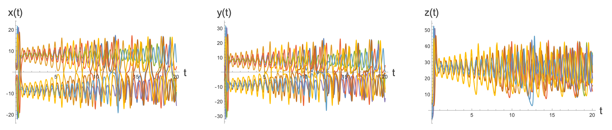
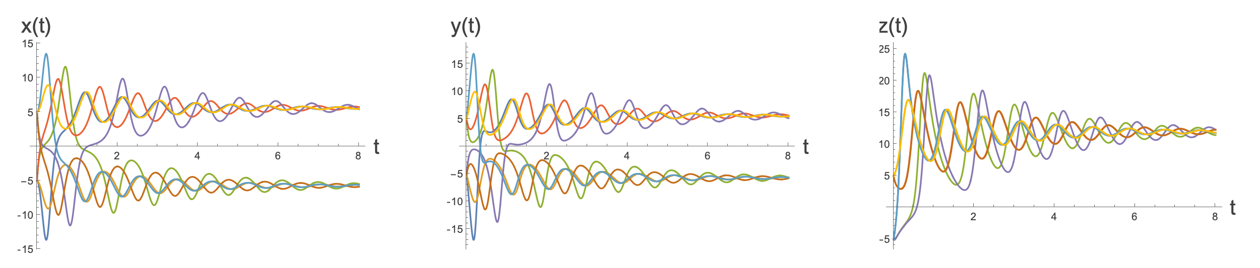
Here we plot the $x, y \text{ and } z $values as a function of time for different starting points in the plane. We see that solutions are attracted to the two fixed points at $C^{\pm{}}.$

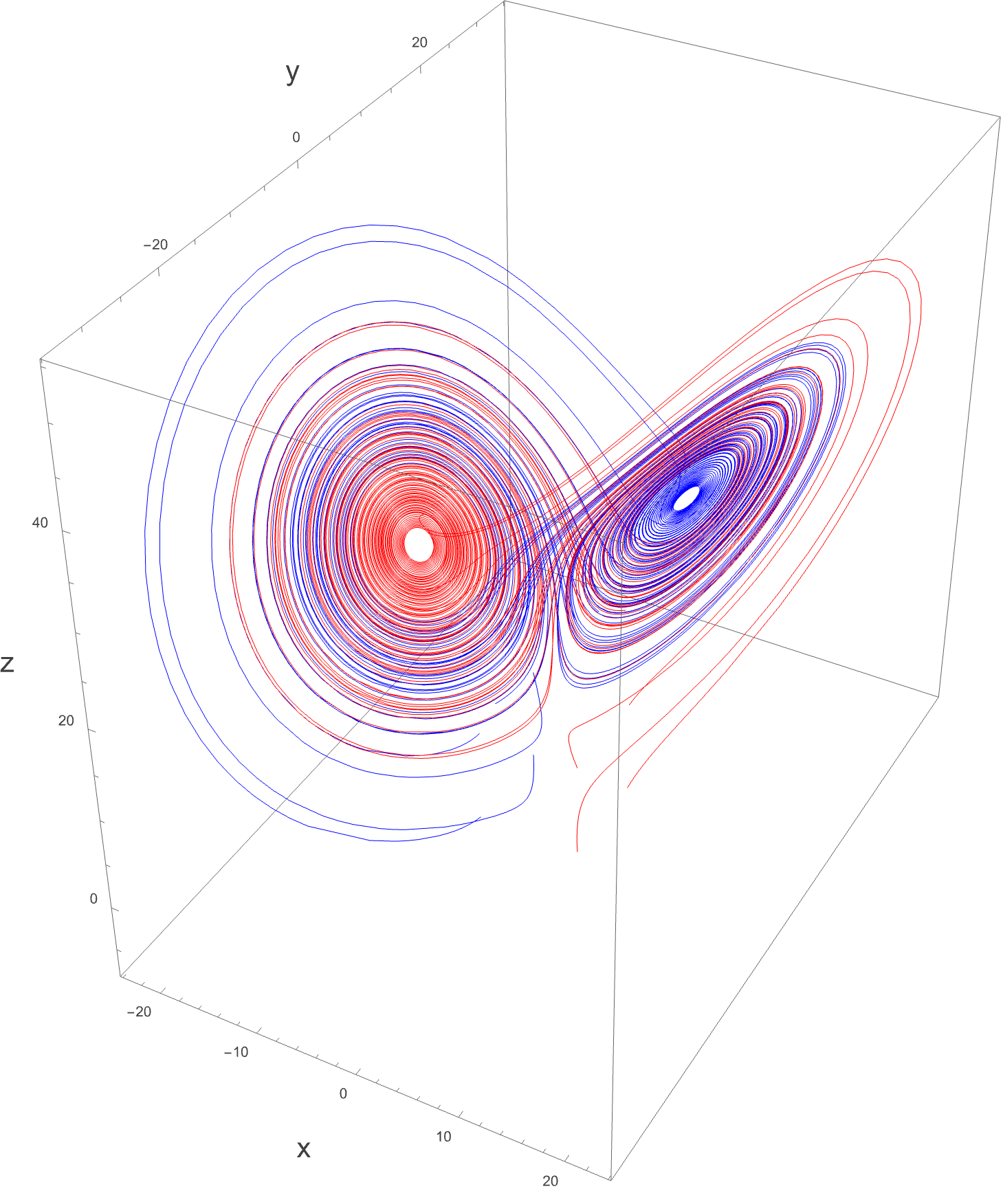
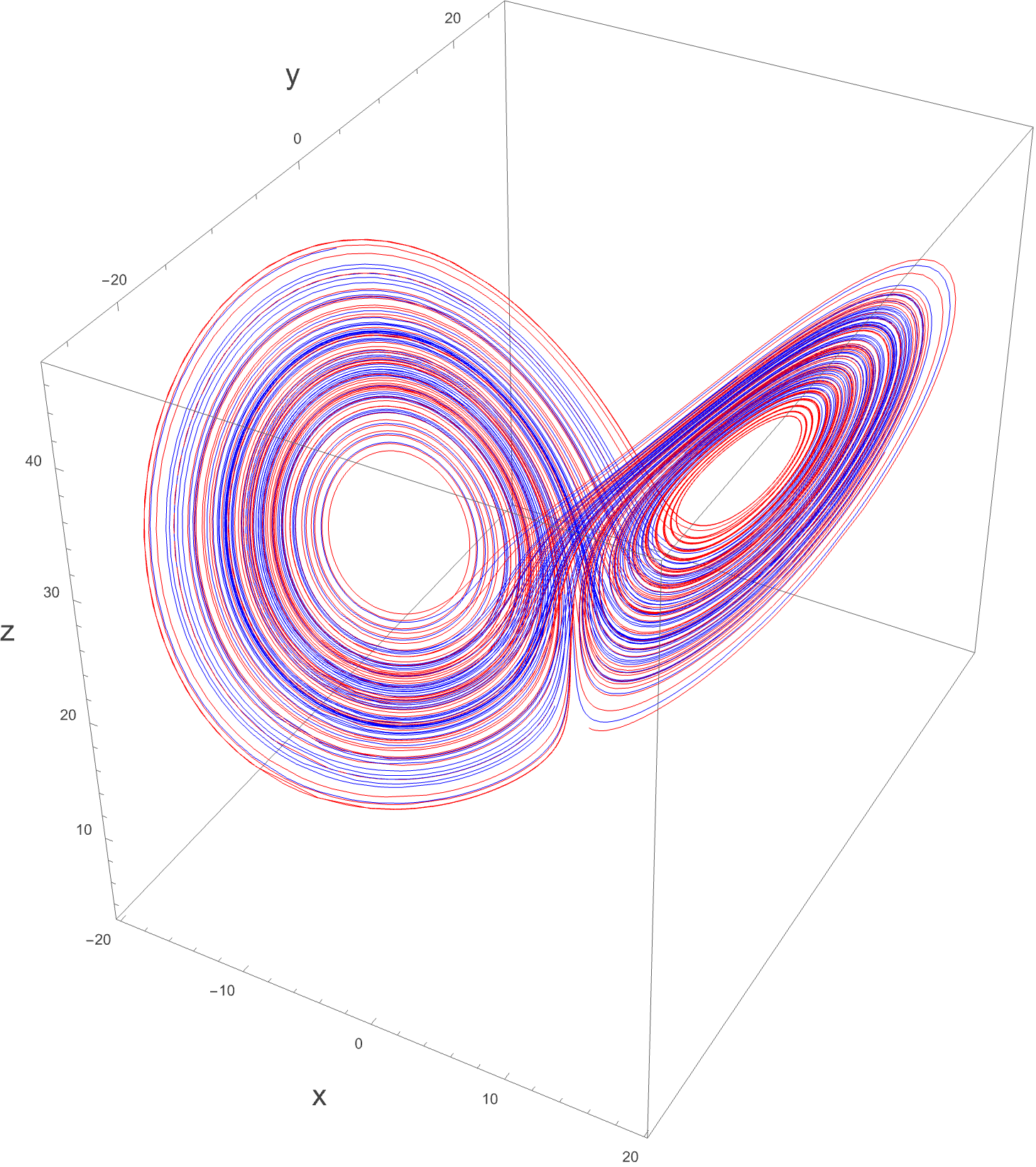
Plotting a few of these in three dimensions we see:

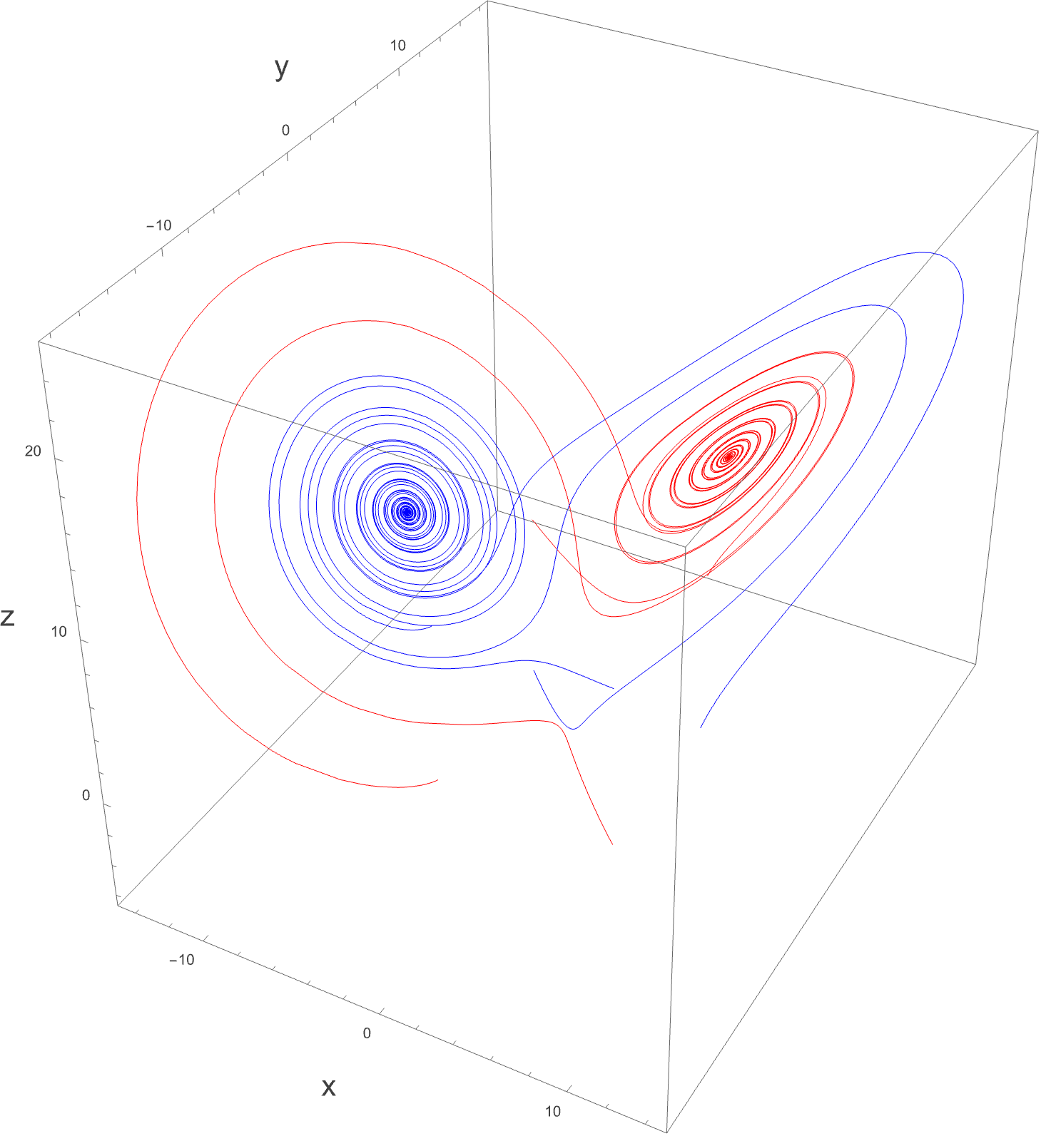
While it might be a little wild, there is no chaos going on here. We can actually create a plot of random starting points and colour them depending on whether they end up at $C^{+} \text{ or } C^{-}$ (themselves denoted as the black points):

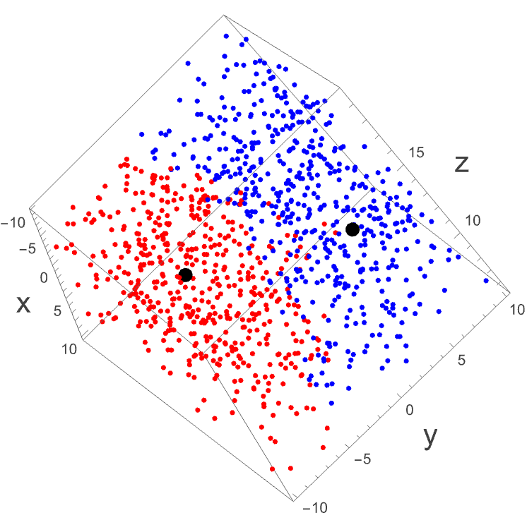
We see that the two groups are pretty well separated. Knowing roughly the region that you start will tell you roughly the region you end up at - which will be one of the two stable fixed points.

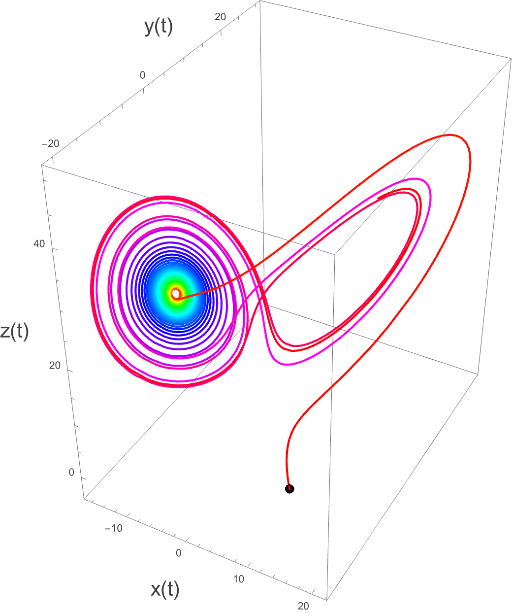
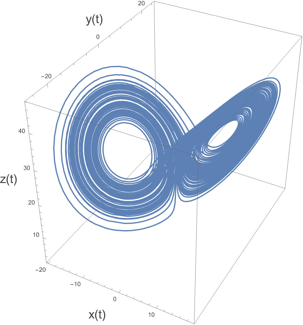
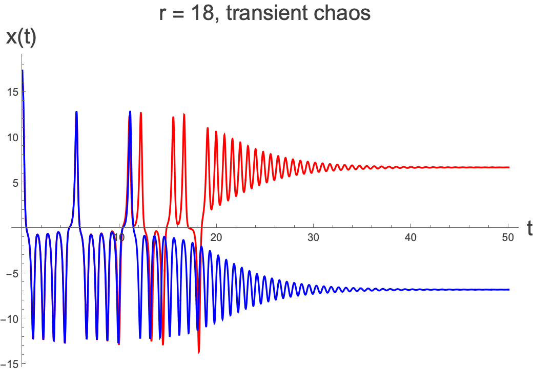
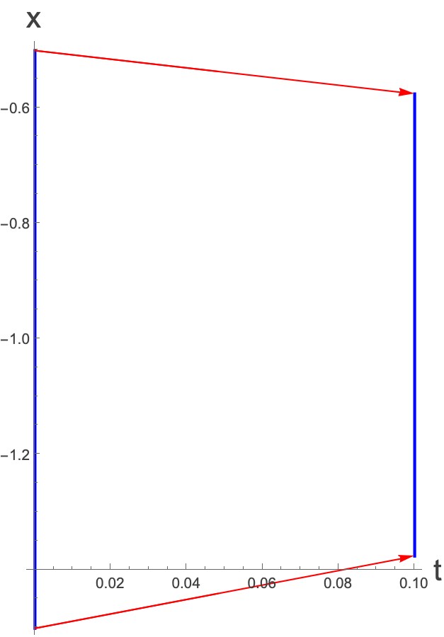
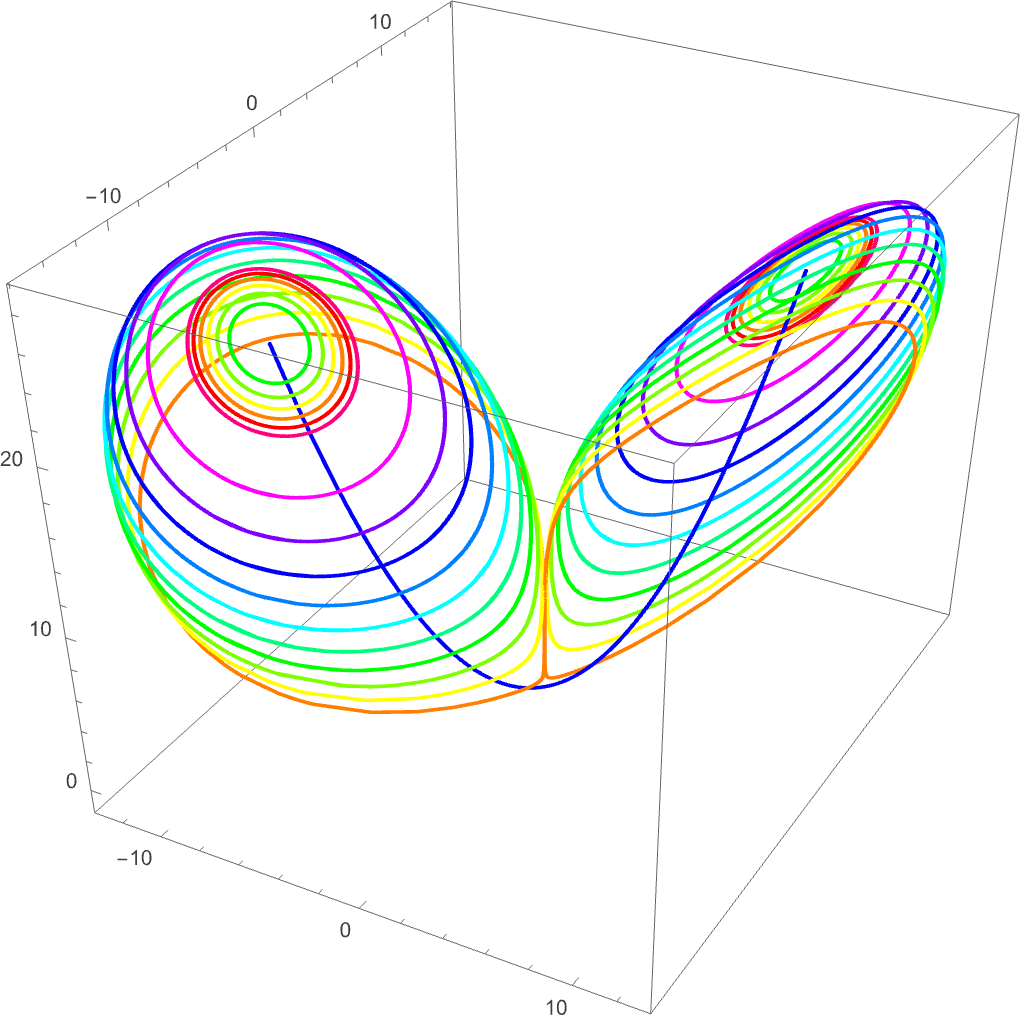
But this is all for $r

It’s actually possible to prove that all trajectories end up within a certain region of the phase space. The argument is akin to a trapping region argument, where the trapping region is an ellipsoid. We are not going to prove it here. What can also be argued is that there are no other stable limit cycles in the system.

So what does this leave? Well, it leaves some sort of attracting region, but one where there are no periodic flows. This is a so-called strange attractor (to be described soon), and is certainly related to the planes in which the unstable limit cycles once inhabited before they collapsed in on the stable fixed points.

Let’s just produce the same plots as before, this time with $r>r_{H}:$

Here we produce the same starting points for the curves as last time, and this time we colour them based on where they started (red if the sign of $x_{0}>0$ and blue otherwise).

What we see here doesn’t look all that different from what we had for a lower value of $r$, however now the blue and red lines seem to be all mixed up. There also appear to be two regions which don’t seem to be that mixed up, in the middle of each ‘disk’. However, these are regions which trajectories are moving away from. If we look at what happens after $t=180 \text{ and up } \text{ to } t=200 $here, we see that none of the trajectories are in these regions close to the unstable fixed points:

What we have here is a so-called strange attractor. It has zero volume, and is like a warped, wrapped surface around the unstable fixed points. All trajectories get attracted to this region, even if they start off way away from it…and yes, now we have chaos. You cannot make predictions about where a trajectory will end up unless you have perfect precision…and you never have perfect precision in reality. Chaos actually requires more than that which we will explore in the next set of notes.

A Strange Attractor, as it is called, is really the far future behaviour (although to simulate it we don’t need to go so far into the future to see what ’s going on. It is called a strange attractor because it attracts all nearby trajectories (in fact in this case all trajectories) over time, and the strangeness is in its fractal properties, which we will take a look at.

Note that the strangeness is often attributed to the chaos, but you can have a nonchaotic strange attractor. The strangeness is really about the structure of the attractor, not about its sensitivity to initial conditions.

Let’s see if we can get a sense of what is going on for a single trajectory.

The color is just to give an idea of where it is, when. The colours go from red to blue through the rainbow and back again.

The trajectory here starts off outside of the Strange Attractor at the position of the black point. It quickly gets swept up and falls down one of the trajectories which previously was part of the stable direction leading into the stable fixed point surrounded by the unstable limit cycle. It then slowly makes its way around the plane where the unstable limit cycle used to be (see transient behaviour, below). It spirals slowly out until it starts to feel the effects of the other plane which corresponded to the previous other unstable limit cycle. This perturbs the trajectory and eventually it gets swept up by that second spiral, spins around that once, comes back to the first, then back to the second, etc. We see essentially that it is the interaction of these two regions that gives rise to the chaotic behaviour. The number of times that it goes around each spiral is itself not predictable and can be used to generate random numbers.

If we take the above single trajectory and run it again far into the future we see:

Again, we have settled into the strange attractor, and always stay away from those central regions, which now contain unstable fixed points.

Let’s look a little more at the transition into chaos by looking at $x\left(t\right)$ for starting positions $\left(0,1,0\right)$ and $\left(0,1.01,0\right)$ as $r$ increases:

We see clearly the incredible sensitivity to initial conditions once we reach the chaotic regime. Just a tiny difference in the starting position leads to completely different behaviours after a relatively short time.

Another thing that we see is that in the chaotic regime, there is still some seemingly periodic behaviour. In fact this is so-called transient behaviour and it happens on the approach to the strange attractor. Once we get close to the strange attractor itself, then the chaos really begins. The transient behaviour is actually observable in the early time trajectory with the arrow pointing to it here:

The above trajectories of $x\left(t\right) $for different values of $r$ do not quite tell the whole story. We’ve actually lied a little…we have essentially said that chaos only appears after $r_{H}$. This isn’t quite true. This is just the point at which the fixed points $C^{\pm{}}$ become unstable. Before that we can still have extreme sensitivity to initial conditions, and the limit cycles which are very close to one another can still mean that we go around the orbits in chaotic ways…but we will still end up at one of the fixed points. Just as we can have transient quasiperiodicityso we can have **transient chaos.**Let’s see if we can spot this transient chaos by starting in the region close to the limit cycles. Here, starting close to $\left(17.4,11.6,10\right)$ we find some transient chaos.

Here the initial conditions differ by just 0.0001, and while they both settle down to the fixed points, they end up at different ones because of the initial region of transient chaos caused by being close to the unstable limit cycles. As we will see, while this is in some colloquial sense chaotic, by the definition that we’ll write down shortly, because you end up at the fixed points in the long time limit, it’s not strictly chaos. It is however very sensitive to initial conditions.

There is one more (actually there are a lot more) subtlety related to the strange attractor. It didn’t actually suddenly appear at the Hopf Bifurcation point. It had been there for a while. In fact it appears at around $r=24.06$ in for the value of $b$ and σ that we’ve been playing with. The transient chaos that occurs takes longer and longer to die down to the fixed points, and at $r=24.06, $the time it takes to die down goes to ∞ and this is when the strange attractor appears. Between $24.06

We have spoken a lot about chaos within this section, and waved our hands about, talking about extreme sensitivity to initial conditions…can we be any more concrete here? Well, we will look into trying to pin down chaos a bit more quantitatively in the next section. We will also talk a little more about the structure of the strange attractor and quite why it is a fractal.