Section 3.6: Poincaré maps

Section 3.6: Poincaré maps

We’re now going to introduce one of the key methods which will be needed for studying chaos later in the course. It’s a way to get a picture of what is happening in a phase portrait in potentially higher dimensional systems where just looking at the phase portrait as we have studied it so far is going to be too complicated.

We’re going to start off with an example and see how we can generalise. We’re going to take a relatively simple system, of the form:

$$ \dot{r}=r\left(1-r^{2}\right) $$$$ \dot{\theta{}}=5 $$

and let’s start off with initial condition $\theta{}\left(0\right)=0, r\left(0\right)=0.1$. We can easily plot the trajectory for this flow as we can actually solve this system analytically:

$$ \int{}\frac{1}{r\left(1-r^{2}\right)}\mathrm{d}r =\int{}\mathrm{d}t \Longrightarrow{} r\left(t\right)=\frac{0.1{\mathrm{e}}^{t}}{\sqrt{{0.1}^{2}\left({\mathrm{e}}^{2 t}-1\right)+1}} $$$$ \overset{ }{\theta{}}\left(t\right)=5t $$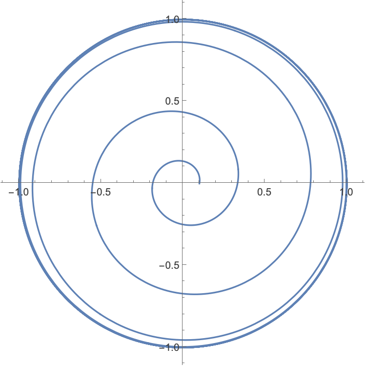

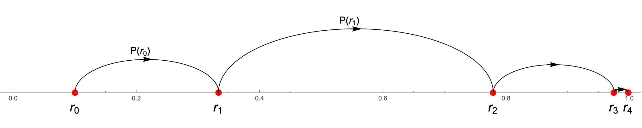
We can ask what we would see if we were just sitting on the positive x-axis. Every $\frac{2\pi{}}{5}$ we would see the path whizz past again. We will call the positive x-axis the surface of section, and label it $S.$ In general we will be interested in creating some surface $S$ (which in this case is actually just a line, but in higher dimensions it can be a surface, or hypersurface), and asking about how a trajectory intersects with this surface. It’s important also that the trajectories don’t flow along the surface, but pass through it. Let’s see what happens from the point of view of the surface in this case.

We start on the surface at position $r_{0}=0.1$. On the next pass through, we have been travelling for time t=$\frac{2\pi{}}{5}$, so we are now at

$$ r_{1}= r\left(\frac{2\pi{}}{5}\right)=\frac{0.1{\mathrm{e}}^{\frac{2\pi{}}{5}}}{\sqrt{{0.1}^{2}\left({\mathrm{e}}^{\frac{4\pi{}}{5}}-1\right)+1}}=0.33297730042280477` $$

On the next rotation we are at

$$ r_{2}= r\left(\frac{4\pi{}}{5}\right)=\frac{0.1{\mathrm{e}}^{\frac{4\pi{}}{5}}}{\sqrt{{0.1}^{2}\left({\mathrm{e}}^{\frac{8\pi{}}{5}}-1\right)+1}}=0.7785979093737593` $$

We define a map $P$ which takes us from $r_{i} \text{ to } r_{i+1}:$

$$ r_{i+1}=P\left(r_{i}\right) $$

So we can imagine that this map takes a point on $S$ and maps it to a new point on $S:$

Clearly this will carry on forever and the points will get closer and closer together as we go around more and more times.

Congratulations, you have just seen your firstPoincaré map, though this isn’t the usual way that it’s presented. This is really to make sure that we can see why it’s a map.

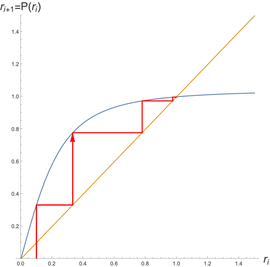
One could think about doing this as a cobweb diagram. To get this we need the mapping P(r) explicitly, but this is just the same as plugging in $r_{i}$ instead of 0.1 into our equation, and asking what is the position after time $\frac{2\pi{}}{5}:$

$$ r_{i+1}=\frac{r_{i}{\mathrm{e}}^{\frac{2\pi{}}{5}}}{\sqrt{{r_{i}}^{2}\left({\mathrm{e}}^{\frac{4\pi{}}{5}}-1\right)+1}} $$

So therefore:

$$ P\left(r\right)=\frac{{r\mathrm{e}}^{\frac{2\pi{}}{5}}}{\sqrt{r^{2}\left({\mathrm{e}}^{\frac{4\pi{}}{5}}-1\right)+1}} $$

Plotting this, with $r_{0}=0.1$ we get the following cobweb diagram, where we have plotted both $P\left(r\right) \text{ and } r$ and we bounce between the two of them.

Again, this is an illustration of the Poincaré map for this system.

We see here (although we knew it already) that there is a unique, globally stable limit cycle at $r^{*}=1$.

Let’s take a step back and think about what we ’ve got here. We took a system where we could define some surface (in this case actually a line) where the trajectories passed through. It happened to be in a relatively simple periodic way in this case, but it doesn’t have to be. We could then define something about the relative positions that the trajectory passed through the surface. This is the map from one pass through to the next, and is what we call the Poincar é map. Each point on the surface gets mapped to another point on the surface. We saw that there was a fixed point on the map, and this corresponds to the stable limit cycle.

Let’s look at another example, this time of the driven system:

$$ \dot{x}+x=A \text{ sin } \omega{} t $$

for some positive driving frequency ω. We can turn this into a two-dimensional autonomous system given by:

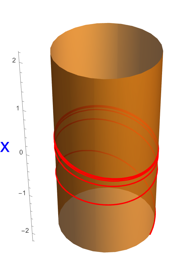
$$ \dot{x}+x=A \text{ sin } \theta{} $$$$ \dot{\theta{}}=\omega{} $$

where this system is periodic in θ with period $\frac{2\pi{}}{\omega{}}$. Note that here we have $x $and θ and not $r \text{ and }$ θ. $r \text{ and }$ θ corresponds to a parameterization of a two dimensional plane in polar coordinates, but $x $and θ do not, because x isn’t constrained to be positive. A simple way to visualise such a phase space is a cylinder:

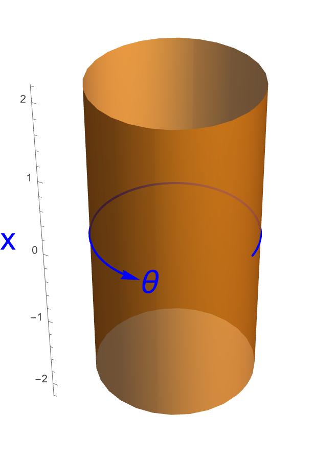
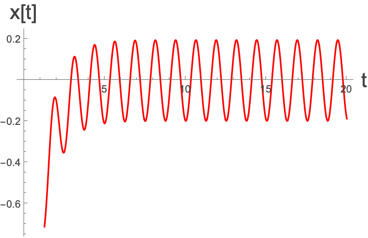
Let’s look at a characteristic trajectory on this surface (we’ll remove the θ arrow for clarity), with $x\left(0\right)=-2$, $\theta{}\left(0\right)=0$. We will also choose $A=1 $and $\omega{}=5.$

Notice that if we were to plot $x\left(t\right) $on its own it would be:

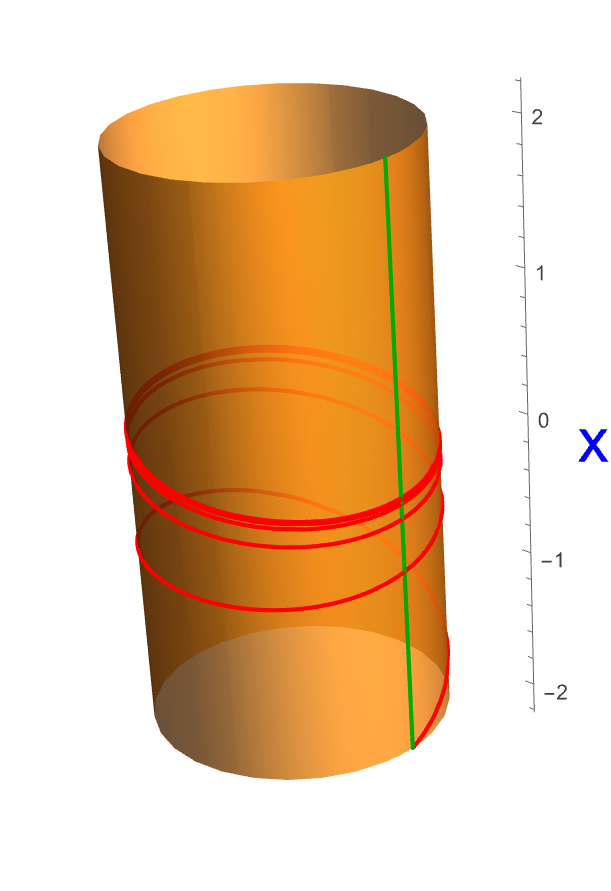
What could we choose for the Surface of Section? Well, actually there are an infinite number of possible choices, but a natural one would be a fixed value of θ - ie a vertical slice through the cylinder. Let ’s take one like this with $\theta{}=0$:

To get the Poincaré map, we can do so numerically, but it ’s much better to do so analytically. The solution to the general differential equation with $x\left(0\right)=x_{0}$ can be shown to be:

$$ x\left(t\right)=\frac{ \left(\left(x_{0}\left(1+{\omega{}}^{2}\right)+A \omega{}\right){\mathrm{e}}^{-t}-A \left(\omega{} \text{ cos }\left(t \omega{}\right)+\text{ sin }\left(t \omega{}\right)\right)\right)}{1+{\omega{}}^{2}}, \theta{}\left(t\right)=t\omega{} $$

The question that we have to ask then is what is $x\left(\frac{2\pi{}}{\omega{}}\right)$. This will be the map that we are interested in.

$$ x\left(\frac{2\pi{}}{\omega{}}\right)=\frac{ \left(\left(x_{0}\left(1+{\omega{}}^{2}\right)+A \omega{}\right){\mathrm{e}}^{-\frac{2\pi{}}{\omega{}}}-A \left(\omega{} \text{ cos }\left(2\pi{}\right)+\text{ sin }\left(2\pi{}\right)\right)\right)}{1+{\omega{}}^{2}}=x_{0}{\mathrm{e}}^{-\frac{2\pi{}}{\omega{}}}+\frac{A \omega{} \left({\mathrm{e}}^{-\frac{2\pi{}}{\omega{}}}-1\right)}{1+{\omega{}}^{2}} $$

So more generally:

$$ P\left(x\right)=x {\mathrm{e}}^{-\frac{2\pi{}}{\omega{}}}+\frac{A \omega{} \left({\mathrm{e}}^{-\frac{2\pi{}}{\omega{}}}-1\right)}{1+{\omega{}}^{2}} $$

Let’s play exactly the same game as before with the cobweb diagram choosing $A = 1 \text{ and } -1, \omega{} = 5,x_{0}=-2 \text{ and } x=2$:

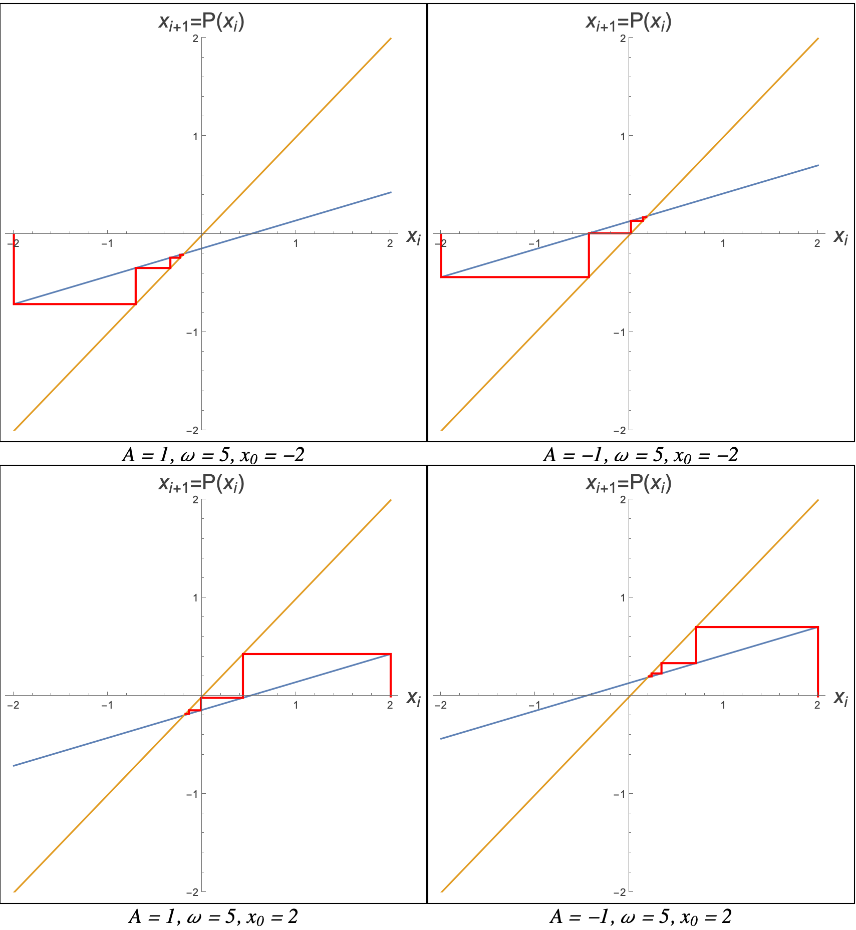
Again, we see here that there is a single, unique, globally stable limit cycle where $P\left(x^{*}\right)=x^{*}$ which is at:

$$ x^{*}=-\frac{A \omega{}}{1+{\omega{}}^{2}} $$

The one thing that we need to be careful of is the gradient of $P\left(x\right)$. It is a straight line, with gradient ${\mathrm{e}}^{-\frac{2\pi{}}{\omega{}}}$. If the gradient is ever equal to one, then the two lines $\left(y=P\left(x\right) \text{ and } y=x\right) $will never intersect. For any other value they will. So we will have a limit cycle unless

$$ e^{-\frac{2\pi{}}{\omega{}}}=1 $$

This can clearly never happen unless $\omega{}\to \infty{}$. Also, because ω is never negative, this will always be between $\left(0,1\right)$. This is very important that the gradient of the line is never greater than 1, for reasons we will see in a little bit.

This whole system actually models a sinusoidally forced resistor-capacitor system, and what the stable limit cycle tells us here is that it we will move towards a regular forced oscillation, however the system may have started off.

Stability of the limit cycle

We can actually use the technology that we’ve just developed to ask about the stability (at least linear stability) of periodic orbits. A fixed point of the Poincaré map is a point $x^{*} $which is mapped to itself

$$ P\left(x^{*}\right)=x^{*} $$

The statement holds true whatever the dimension of the Surface of section, so we can make $x^{*}$ be a vector $x^{*}$ of any system

$$ \dot{x}=f\left(x\right) $$

To be a stable periodic orbit, we should be able to move a little way away from $x^{*} $and check the stability.

If we start a little away from $x^{*}$, for instance at $x^{*}+v_{0}$, for some infinitesimal $v_{0}$, then under the Poincaré map we should have:

$$ x^{*}+v_{1}=P\left(x^{*}+v_{0}\right) $$

we know we won’t end up back at the same place, but we do expect to end up somewhere nearby, $v_{1}$ should also be small. For small $v_{0}$ we can expand P. However, we may be in a multi-dimensional space here and so our Taylor expansion will involve an $\left(n - 1\right)$ x $\left(n-1\right)$ matrix, where $n \text{ is the } $dimension of the phase space. In the cases that we’ve been looking at here therefore this will just be a regular derivative along the surface of sections, as we were in 2d phase spaces. However, in general it will be some matrix of derivatives which we denote as $D P\left(x^{*}\right)$ (this is just the Jacobian of $P $at the fixed point of the map) So we have:

$$ x^{*}+v_{1}=P\left(x^{*}\right)+D P\left(x^{*}\right).v_{0}+O\left(|v_{0}|^{2}\right) $$

where here we have a dot product between the matrix of derivatives acting on $P$ and the vector $v_{0}$. Of course $x^{*}=P\left(x^{*}\right)$ so we have:

$$ v_{1}=D P\left(x^{*}\right).v_{0} $$

In exactly the same way as we have with the Jacobian in a regular linearisation, the stability of this system will be down to the eigenvalues of $D$ $P\left(x^{*}\right)$. However, the criterion is a little different to what we have seen before where we were only interested in the sign of the real part of the eigenvalue.

We can understand what the criterion might be by taking the case where there are no degenerate (ie. repeated) eigenvalues. In this case we will have $n-1$ eigenvectors making up a basis {$e_{i}}$. We can write $v_{0}$ as some linear combination of these (not necessarily orthogonal) basis vectors:

$$ v_{0}=\underset{i=1}{\overset{n-1}{\sum{}}}m_{i}e_{i} $$

where here $m^{i}$ are some set of scalar values, which remember are going to be very small, because the $e_{i}$ will often be a normalised basis, and we need $v_{0}$ to be infinitesimally small.

OK, now taking this and plugging it into the above equation we have:

$$ v_{1}=D P\left(x^{*}\right). \underset{i=1}{\overset{n-1}{\sum{}}}m_{i}e_{i} $$

We can take the matrix inside the summation and take the $m_{i}$ to the front:

$$ v_{1}= \underset{i=1}{\overset{n-1}{\sum{}}}m_{i}D P\left(x^{*}\right).e_{i} $$

and now we have the matrix $D$ $P\left(x^{*}\right)$ applied to $e_{i} $which are eigenvalues of this matrix, with eigenvalues ${\lambda{}}_{i}$, so we have:

$$ v_{1}= \underset{i=1}{\overset{n-1}{\sum{}}}m_{i}{\lambda{}}_{i}e_{i} $$

Remember that the right hand side was essentially a matrix operation on the starting vector (away from the fixed point). We can do this again to get:

$$ v_{2}= \underset{i=1}{\overset{n-1}{\sum{}}}m_{i}{{\lambda{}}_{i}}^{2}e_{i} $$

and in fact we can iterate it any number of times to get:

$$ v_{k}= \underset{i=1}{\overset{n-1}{\sum{}}}{m_{i}\left({\lambda{}}_{i}\right)}^{k}e_{i} $$

When is $v_{k}$ going to go to zero, proving that the fixed point is stable? Well, it will happen so long as all of the eigenvalues have magnitude less than one:

$$ |{\lambda{}}_{i}|<1, \text{ for all } i=1,..., n-1 $$

What happens when $|{\lambda{}}_{i}|=1$ for some eigenvalue? Well, that is a borderline case, and this linear stability analysis fails in that case. In fact you will find that this takes place when there is a bifurcation in a limit cycle.

The ${\lambda{}}_{i}$ that we’ve been talking about are called Floquet or Characteristic Multipliers.

We can think of the Floquet multipliers as telling you how quickly a small perturbation from the orbit will grow or shrink. When you are in higher dimensions, it also tells you the direction that you will be growing/shrinking. Thus, for a two dimensional system, with a one dimensional surface of sections, we have a single Floquet multiplier which tells us how fast we will move towards/away from the limit cycle. In fact, in that case the Floquet multiplier will just be given by:

$$ \lambda{}=P'\left(x^{*}\right) $$

We have to be very careful here not to get confused with the normal type of linear stability analysis where we have some instability growing or shrinking exponentially. Remember we have a map here which can be thought of as a discrete set of steps. The λ tells you about how you grow each time you pass through the surface, so these are a discrete set of jumps. Let ’s go back to the case above and start close to the limit cycle:

The Floquet multiplier in this case is:

$$ \lambda{}=P'\left(x^{*}\right)=\frac{d}{d x}\left(x {\mathrm{e}}^{-\frac{2\pi{}}{\omega{}}}+\frac{A \omega{} \left({\mathrm{e}}^{-\frac{2\pi{}}{\omega{}}}-1\right)}{1+{\omega{}}^{2}}\right)|_{x=x^{*}}=e^{-\frac{2\pi{}}{\omega{}}} $$

which says that if we start close to the fixed point, we will go towards it by a factor $e^{-\frac{2\pi{}}{\omega{}}}$ each iteration. In this case, if we start at

$$ x=x^{*}-0.1=-\frac{A \omega{}}{1+{\omega{}}^{2}}-0.1 $$

then on the next iteration we will be at

$$ x=x^{*}-0.1\lambda{}=-\frac{A \omega{}}{1+{\omega{}}^{2}}-0.1 \lambda{}=-\frac{A \omega{}}{1+{\omega{}}^{2}}-0.1 e^{-\frac{2\pi{}}{\omega{}}} $$

and on the next at

$$ x=x^{*}-0.1{\lambda{}}^{2}=-\frac{A \omega{}}{1+{\omega{}}^{2}}-0.1 {\lambda{}}^{2}=-\frac{A \omega{}}{1+{\omega{}}^{2}}-0.1 e^{-\frac{4\pi{}}{\omega{}}} $$

etc. Let’s test this hypothesis by plotting this values as green points with $x$-values given above, and $y$-values given by $x^{*}$, just for illustrative purposes.

Looks good to me!

In fact in this case, because the Poincaré map is a straight line, the linearisation is exact for any starting value.

So just don’t think that the linear term gives you some continuous time behaviour of perturbations away from or towards the fixed point, we are talking about iterated maps here.