Section 3.5: Coupled oscillators and quasiperiodicity
Section 3.5: Coupled oscillators and quasiperiodicity
When we discussed the phase space of the pendulum in first year, we said that we were free to choose $\theta{}\left(0\right)$ and $\dot{\theta{}}\left(0\right)$, which is indeed true, but we ended up plotting trajectories in phase space like:
(where here $x_{1} \text{ is } \theta{}$ and $x_{2} \text{ is }$ $\dot{\theta{}}$). We never took into account the fact that θ is periodic (though $\dot{\theta{}}$ is of course not) - ie $\theta{}+2\pi{} \text{ is identified } \text{ with } \theta{}$. The way we should do this is to acknowledge that the phase plane shouldn ’t be ${\mathbb{R}}^{2}$ but it should be ${\mathbb{R}}^{1}\times{}S^{1}$ - ie a cylinder.
Imagine taking the first plot and pasting it around a cylinder of circumference 2π.
OK, so here we have an example when a phase plane is most naturally described as a phase cylinder. Are there other systems for which we might have a different description?
We know that in a one dimensional system we can’t have any oscillations in terms of a back and forth motion, but of course we can have a flow on the line, where there is an identification on the line meaning that it’s really on a circle. Such a flow would be given by:
$$ \dot{\theta{}}=f\left(\theta{}\right) \text{ with identification } \theta{}+2\pi{}\sim{}\theta{} $$where the [Tilde] symbol means “is identified with ”. This is really a flow on a circle.
We can do the same thing in two dimensions, and think about having two coupled oscillators (flows on a circle), given by, for instance
$$ \dot{{\theta{}}_{1}}={\omega{}}_{1}+K_{1}\text{ sin }\left({\theta{}}_{2}-{\theta{}}_{1}\right) $$$$ \dot{{\theta{}}_{2}}={\omega{}}_{2}+K_{2}\text{ sin }\left({\theta{}}_{1}-{\theta{}}_{2}\right) $$Where ${\omega{}}_{1}\text{ and } {\omega{}}_{2} \text{ are } $the natural frequencies of the motion (ie. without the $K_{i} \text{ terms }$ we would just have ${\theta{}}_{i} \text{ going }$ around a circle at frequency ${\omega{}}_{i}$), and $K_{i} \text{ are }$ coupling constants. We see then that when ${\theta{}}_{1} \text{ and } {\theta{}}_{2}$ are very close to each other, or differ by π, the couplings are small, and when they differ by $\frac{\pi{}}{2} \text{ or } \frac{3\pi{}}{2}$ the couplings are large. This system wants to keep the ${\theta{}}_{i} \text{ close to } $each other, or exactly out of phase. Both the ${\theta{}}_{i} \text{ live }$ on a circle. We can plot them on the same circle and see their trajectory. For instance if we start with ${\omega{}}_{1}=1$, ${\omega{}}_{2}=5$ and both $K_{i}=1 $we get:
Is there a simpler way that we could illustrate this? We normally like to think about the state of a system as a single point in phase space. The problem with the above is that we have a single state as being given by two points on the circle. The issue is that we have a two dimensional phase space and we are trying to represent it on a one dimensional space. So what we really need is a space with two compact directions. Such a space is the torus. In the above, we have a state given by two points $\left({\theta{}}_{1}\left(t\right),{\theta{}}_{2}\left(t\right)\right).$ The torus is a surface which is parameterised by $\left({\theta{}}_{1}\left(t\right),{\theta{}}_{2}\left(t\right)\right). $So for two points on the circle corresponds to a single point on the surface of the torus.
The torus is actually given by the product space $S^{1}\times{}S^{1}$, which is like having two independent circles. One way to see this is to take a piece of paper and first identify the left and right opposite sides. You’ve now got one circular direction. Now do the same thing with the top and bottom (actually, this will be hard with paper as it ’s not stretchable) and you have two circular directions.
Taking the above system of two positions on the circle $\left({\theta{}}_{1},{\theta{}}_{2}\right) \text{ and }$ converting them to one position on the torus, we get the following trajectory:
Where the trajectory through phase space maps out a line on the surface of the torus. One could imagine unfolding the square, and just plotting positions in the $\left({\theta{}}_{1},{\theta{}}_{2}\right)$ square. Try it for yourself…
This particular case is an example of a general form of a vector field which lives on a torus. That of
$$ \dot{{\theta{}}_{1}}=f_{1}\left({\theta{}}_{1},{\theta{}}_{2}\right) $$$$ \dot{{\theta{}}_{2}}=f_{2}\left({\theta{}}_{1},{\theta{}}_{2}\right) $$with a natural identification of ${\theta{}}_{i}+2\pi{}\sim{}{\theta{}}_{i}$.
Going back to the coupled oscillator, there are a couple of interesting limits we can look in.
The first is to ask what happens if the system is not coupled at all. Well, then we get two particles moving around the circle at their own rate, say 1:
$$ \dot{{\theta{}}_{1}}=1 $$$$ \dot{{\theta{}}_{2}}=1 $$Clearly if they are both moving at the same rate, then not only is each particle’s trajectory periodic with period 2π, but in fact after 2π, the whole system is back to where it started. How about where we have
$$ \dot{{\theta{}}_{1}}=2 $$$$ \dot{{\theta{}}_{2}}=1 $$well, here, although the first has period π and the second has period 2 π, it takes 2π for the whole system to get back to where it started, although the first oscillator has been around twice by this point. What about if we had
$$ \dot{{\theta{}}_{1}}=2 $$$$ \dot{{\theta{}}_{2}}=3 $$Well, in this case the first has period $\frac{2\pi{}}{2}=\pi{}$ and the second has period $\frac{2\pi{}}{3}.$ After the first has been around once, the second has been around one and a half times, and by the time the second one has been around once, the first has only been around 2/3 of a time. So in fact here we have to wait for a time of 2 π, after which the first oscillator has travelled round exactly twice, and the second has travelled round exactly three times in order to get back to where we started. Plotting these two together, and choosing that they both start off at ${\theta{}}_{i}\left(0\right)=0$ we have:
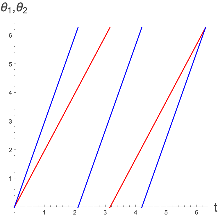
We have to be very careful with what is going on in this plot. ${\theta{}}_{1} \text{ and } {\theta{}}_{2}$ are both increasing at constant rates with $t.$ When they reach 2π, they come back to 0 and continue. We are interested in the point that they are both at ${\theta{}}_{1}={\theta{}}_{2}=2\pi{} $or equivalently 0. This happens after 6π.
Plotting this on the $\left({\theta{}}_{1},{\theta{}}_{2}\right) \text{ plane we } \text{ have }$:
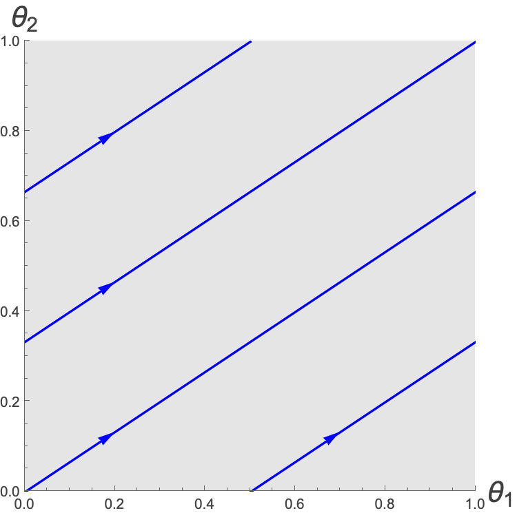
Plotting this on the torus we see:
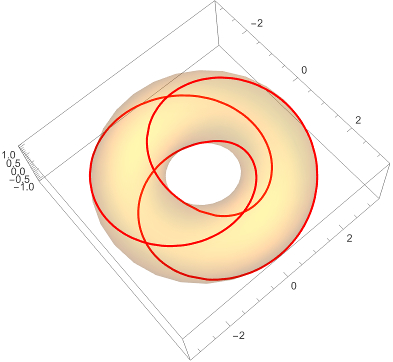
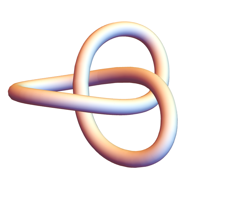
The path that the trajectory makes on the torus is the so-called trefoil knot, which, if we turn the trajectory into a tube to make it easier to visualise, looks like:
In fact we can make a more general statement. If we have two frequencies
$$ \dot{{\theta{}}_{1}}={\omega{}}_{1} $$$$ \dot{{\theta{}}_{2}}={\omega{}}_{2} $$where $\frac{{\omega{}}_{1}}{{\omega{}}_{2}}=\frac{p}{q}\in{}\mathbb{Q}, $where $p\perp{}q$, then the system will be periodic. What will the period be? Well, the period of the first cycle is $\frac{2\pi{}}{{\omega{}}_{1}} $and that of the second is $\frac{2\pi{}}{{\omega{}}_{2}}$. We want to find the lowest positive T such that T=$\frac{2 \pi{}}{{\omega{}}_{1}}p=\frac{2\pi{}}{{\omega{}}_{2}}q$ for $q,p\in{}$ ℤ. In the example above, we had:
$$ T=\frac{2\pi{}}{2}p=\frac{2\pi{}}{3}q \text{ for } p=2,q=3, \text{ therefore } T=2\pi{}. $$If $\frac{{\omega{}}_{1}}{{\omega{}}_{2}}$is not rational, then the system will be quasiperiodic. This is a bit of a strange name because overall the system will never return to its starting position, but the rotation around each cycle of the torus independently is periodic. This means that you will just keep going around the torus forever and never get back to where you started. More than this we can say that the trajectories are dense on the torus. This means that if you pick any point on the torus and any finite number $0 Now let’s extend this very very simple system and allow for a coupling between the two oscillators. We can still talk about the phase space on the torus, but now the trajectories are not just going to wind around each cycle in a way dictated purely by ${\omega{}}_{i}.$ Reminding ourselves of the system, we have: We see here that the coupling is only dependent on the distance between the ${\theta{}}_{i}.$ Let’s subtract the equations from one another: So now we can define a new variable $\phi{}={\theta{}}_{1}-{\theta{}}_{2}$ and rewrite this equation as: Somehow we have a system where the natural frequency is given by the difference between the original frequencies, and the new “coupling” is additive in the old couplings. This system is known as the non-uniform oscillator. Remember, given that φ is the difference between the ${\theta{}}_{i}$ and the coupling only becomes important when the ${\theta{}}_{i} \text{ are far } \text{ apart } $(difference far away from 0 or π), this equation makes sense. What do we do when we are looking at dynamical systems? We ask about the fixed points! The fixed points are clearly given by Well, this only has solutions when and given that $K_{i}$ are positive integers, we have: In fact there will be exactly two fixed points for
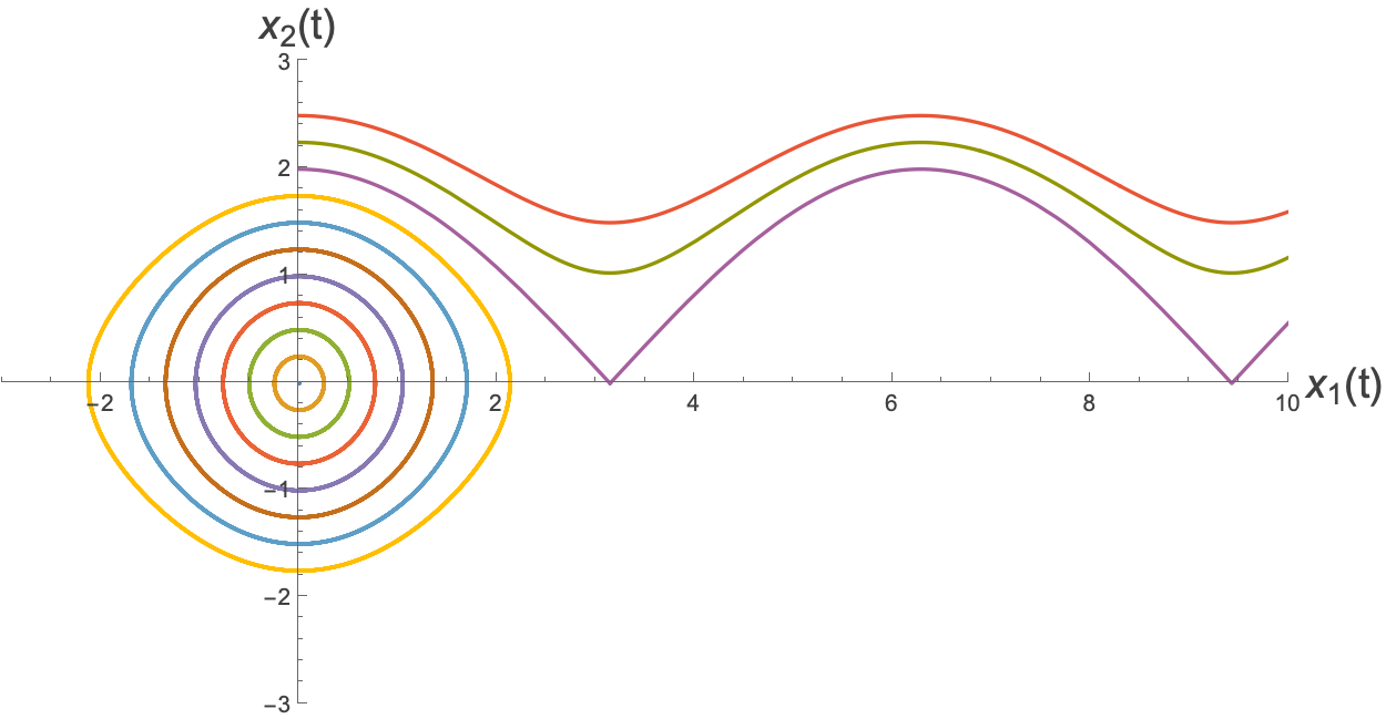
Fixing $K_{1}+K_{2}=1$, and letting ${\omega{}}_{1}-{\omega{}}_{2}=\Delta{}\omega{}$ we have the phase portraits (excluding the arrows):
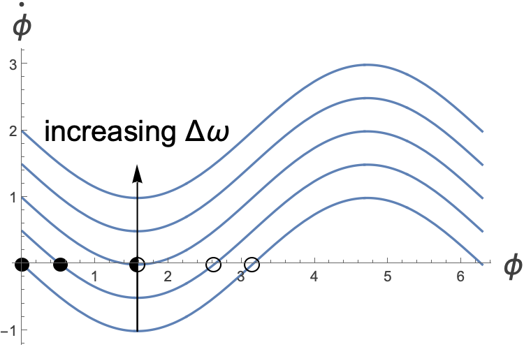
Which looks very much look a saddlenode bifurcation…I rephrase…it is a saddlenode bifurcation.
What does this mean for the case where there are two fixed points? Well, it means that over time $\phi{}\to {\phi{}}^{*}$ which is some constant given by:
$$ \text{ sin }\left({\phi{}}^{*}\right)=\frac{{\omega{}}_{1}-{\omega{}}_{2}}{K_{1}+K_{2}} $$which says that ${\theta{}}_{1}-{\theta{}}_{2}$ tends to this constant. Which means that the two oscillators lock in sync. It doesn’t mean that the two ${\theta{}}_{i}$ are the same, but that their difference becomes constant…they follow each other around the loop at a constant distance. The frequency with which they go around the loop is found by just plugging the above into the original equations:
$$ \dot{{\theta{}}_{1}}={\omega{}}_{1}-K_{1}\text{ sin }\left({\phi{}}^{*}\right)={\omega{}}_{1}-K_{1}\frac{{\omega{}}_{1}-{\omega{}}_{2}}{K_{1}+K_{2}}=\frac{K_{2}{\omega{}}_{1}+K_{1}{\omega{}}_{2}}{K_{1}+K_{2}} $$$$ \dot{{\theta{}}_{2}}={\omega{}}_{2}+K_{2}\text{ sin }\left({\phi{}}^{*}\right)={\omega{}}_{2}-K_{2}\frac{{\omega{}}_{1}-{\omega{}}_{2}}{K_{1}+K_{2}}=\frac{K_{2}{\omega{}}_{1}+K_{1}{\omega{}}_{2}}{K_{1}+K_{2}} $$Thankfully both give the same frequency of
$$ {\omega{}}^{*}=\frac{K_{2}{\omega{}}_{1}+K_{1}{\omega{}}_{2}}{K_{1}+K_{2}}=\frac{K_{2}}{K_{1}+K_{2}}{\omega{}}_{1}+\frac{K_{1}}{K_{1}+K_{2}}{\omega{}}_{2} $$this frequency is known as the compromise frequency and is like a weighted average of the two frequencies, in a weighting related to the relative strengths of the couplings. If $K_{2}$ is much larger, then the frequency of the first oscillator will dominate, and vice versa. Take the case of very large $K_{2}$, very small $K_{1}$, then our equations are approximated by
$$ \dot{{\theta{}}_{1}}={\omega{}}_{1} $$$$ \dot{{\theta{}}_{2}}=K_{2}\text{ sin }\left({\theta{}}_{1}-{\theta{}}_{2}\right) $$Then the first oscillator will have its frequency fixed, and the second oscillator will move towards the point where ${\theta{}}_{2}$ is close to ${\theta{}}_{1}$which means that its frequency is also fixed. With
$$ \dot{{\theta{}}_{1}}=1+0.1\text{ sin }\left({\theta{}}_{2}-{\theta{}}_{1}\right), {\theta{}}_{1}\left(0\right)=0 $$$$ \dot{{\theta{}}_{2}}=3+10\text{ sin }\left({\theta{}}_{1}-{\theta{}}_{2}\right), {\theta{}}_{2}\left(0\right)=2 $$we have the following trajectories
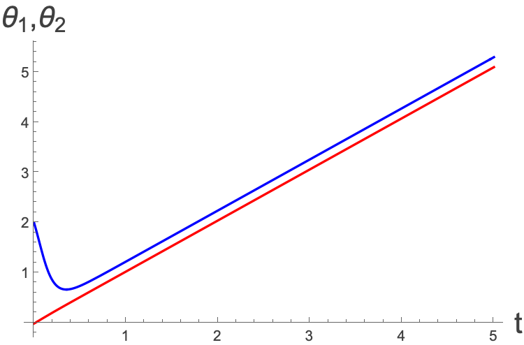
If we have
$$ |\left({\omega{}}_{1}-{\omega{}}_{2}\right)| >K_{1}+K_{2} $$then there is no fixed point, and no phase locking. You can see here that the lines keep crossing each other.
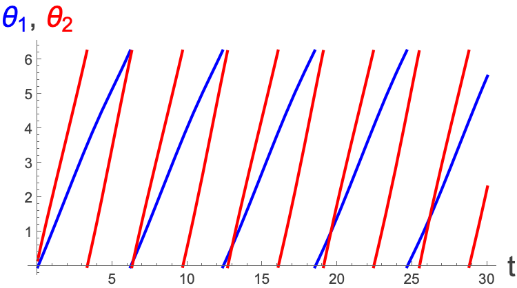
The boundary between the phase locked dynamics and the non phased locked dynamics is a saddlenode bifurcation of cycles.
Explore what sort of behaviour you can get within the $\left({\omega{}}_{1},{\omega{}}_{2},k_{1},k_{2}\right)$ parameter space.