Section 3.4: Global bifurcations of cycles

Section 3.4: Global bifurcations of cycles

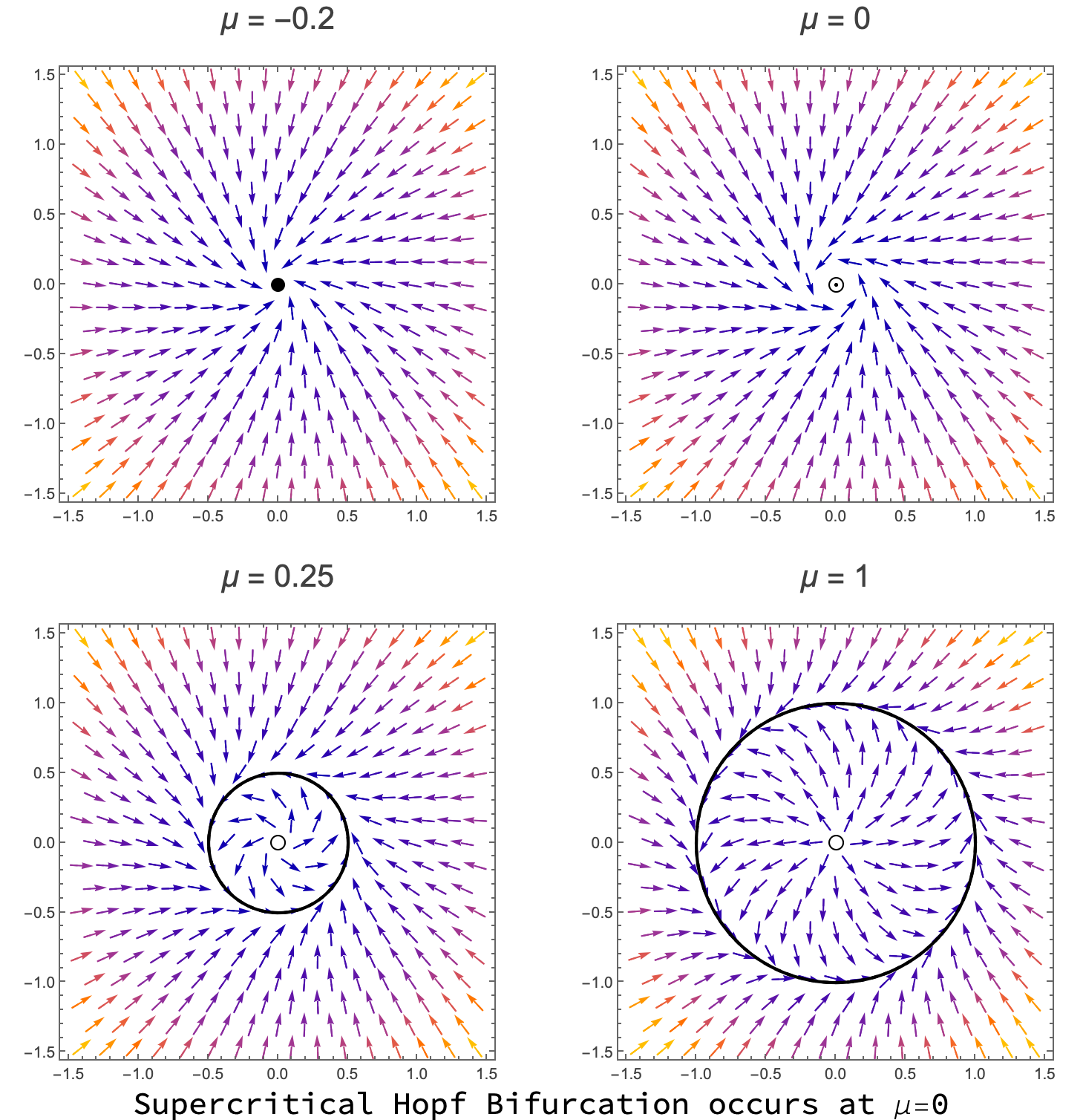
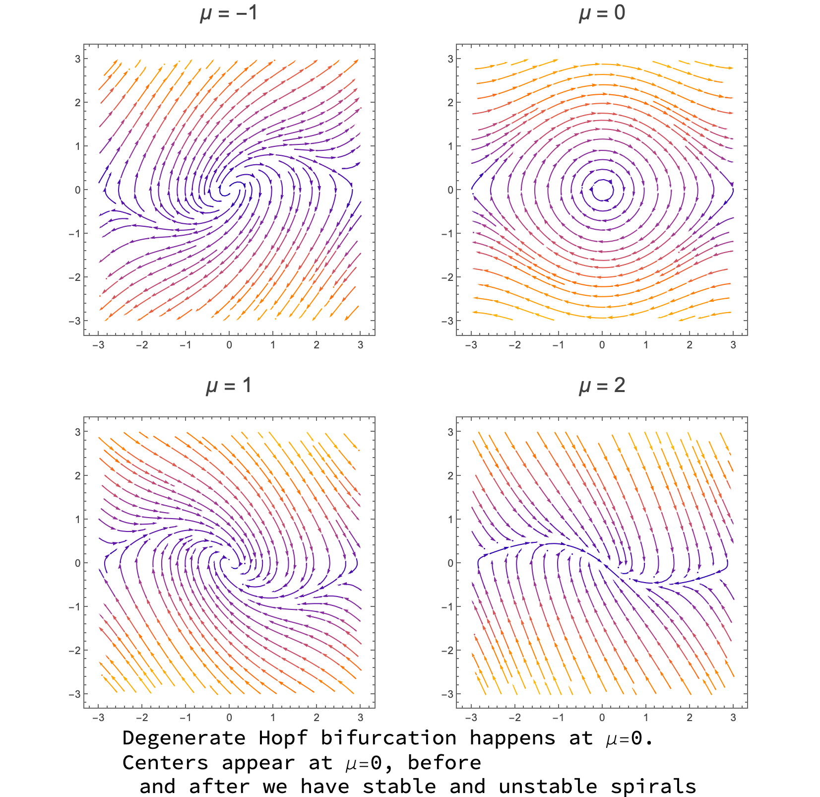
We’ve now seen that while the normal types of bifurcations from 1d persist in 2d and don’t give us anything very different, the existence of limit cycles gives us something more interesting. So far we’ve looked at Supercritical Hopf bifurcations, by which a stable fixed point can explode out into a stable limit cycle and an unstable fixed point, or in the case of the subcritical Hopf bifurcation, an unstable limit cycle can engulf a stable fixed point to become an unstable fixed point. Finally we saw degenerate Hopf bifurcations where there are no limit cycles but only centers about the fixed point which changes from a stable to an unstable spiral across the bifurcation.

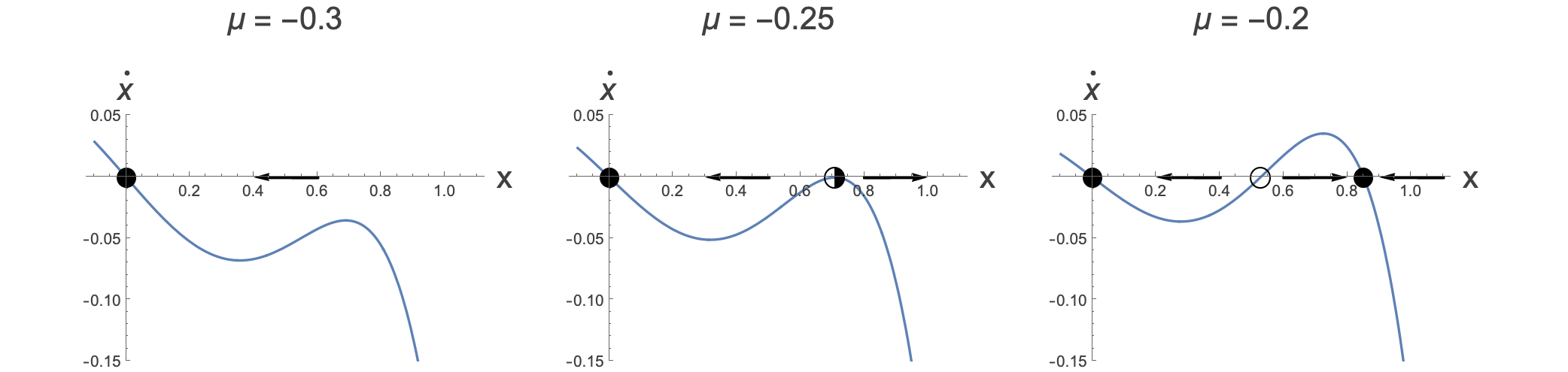
So, what else can happen beyond these bifurcations? For the first case we think about what can happen with a flow on the line, and in particular a saddlepoint bifurcation. This occurs when a stable and unstable fixed point appear out of the blue and move away from one another (generically). An example of this would be

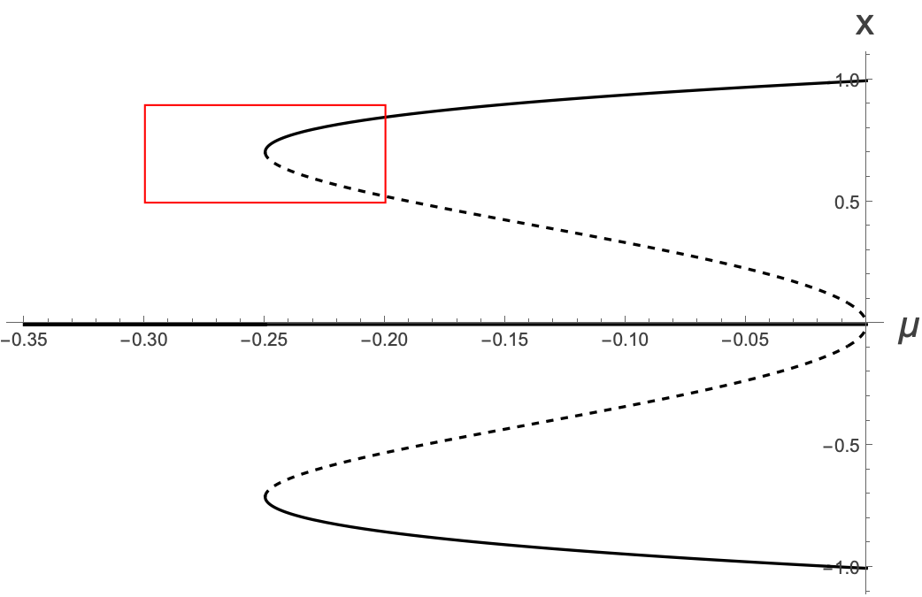
$$ \dot{x}=\mu{} x+x^{3}-x^{5} $$

Which has phase portraits:

Where we are interested in the red box in the bifurcation diagram:

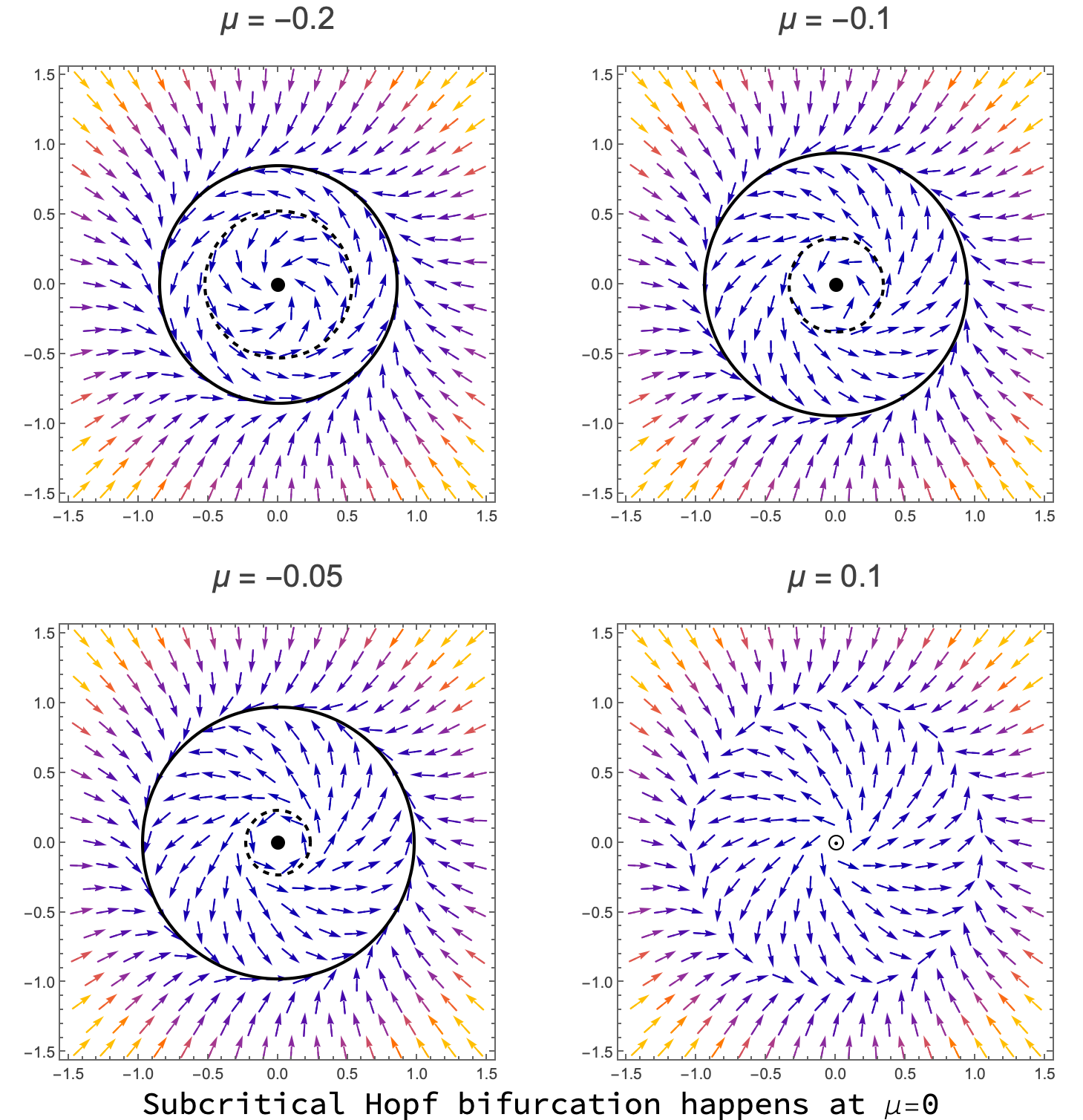
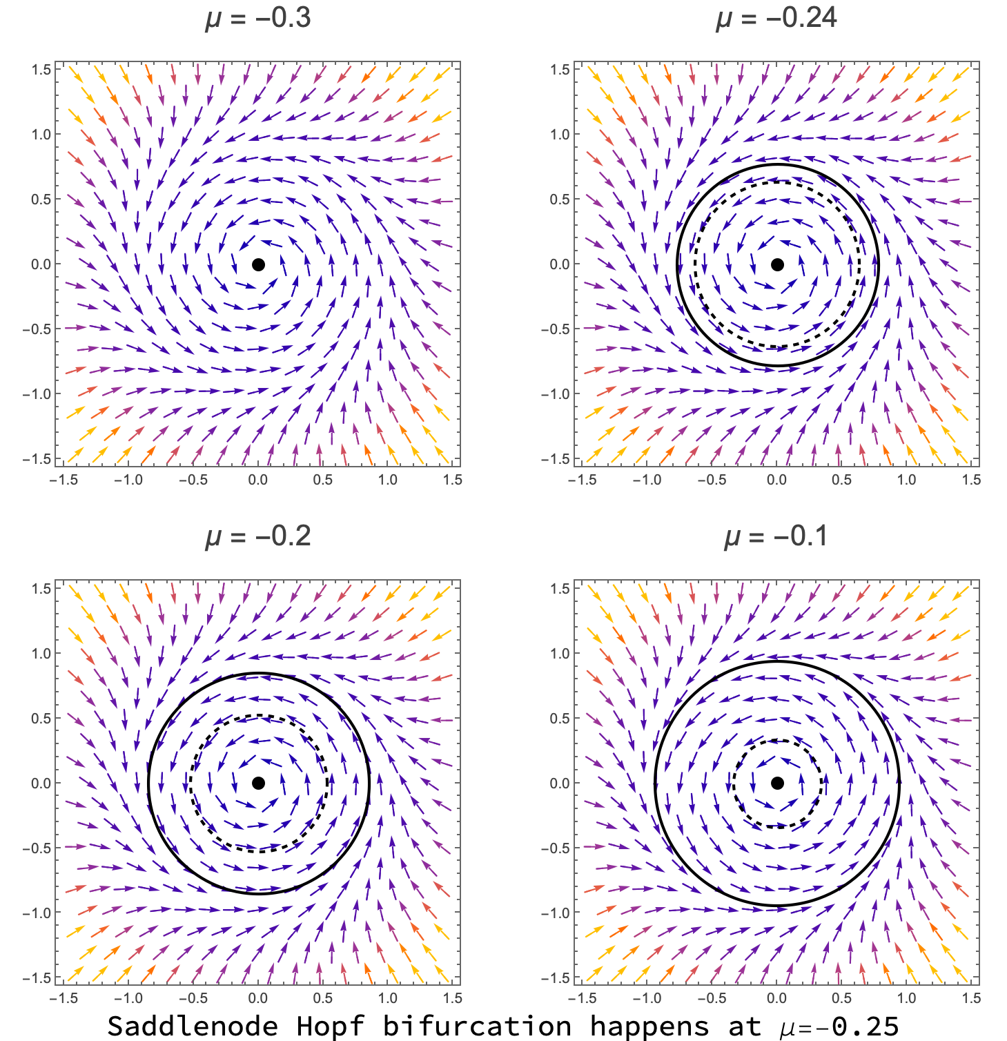
What has this got to do with limit cycles? Well, how about the vector field:

$$ \dot{r}=\mu{} r+r^{3}-r^{5} $$$$ \dot{\theta{}}=\omega{}+b r^{2} $$

Well, this will have exactly the same appearance of a pair of fixed points appearing at finite $r \text{ at }$ a particular value of μ, but we also see that the solutions will have angular velocity. In fact, this is exactly the same case that we illustrated for the subcritical Hopf bifurcation. That happens when $\mu{}=0 $, as indeed happens in the one-dimensional system. The saddlenode Hopf bifurcation occurs at $\mu{}=\frac{-1}{4}$

So this system exhibits both a subcritical and saddlenode Hopf bifurcation, we can see them both happening here

ok, so what else can happen? This one is a little more complicated. Let ’s look at the system (for $\mu{}\geq 0$)

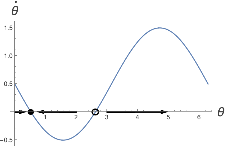
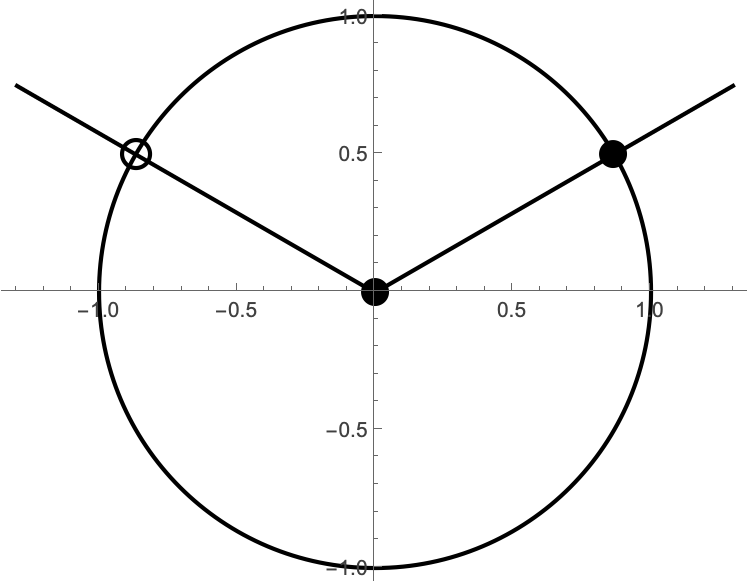
$$ \dot{r}=r\left(1-r^{2}\right) $$$$ \dot{\theta{}}=\mu{}-\text{ sin }\left(\theta{}\right) $$

We see that if you are on the line $r=1$ you will necessarily remain on it. But it’s not right in this case to say that it’s necessarily a closed orbit, or indeed a limit cycle. For $\mu{}>1,$ the second equation has no zeroes, and so there is no angle for which there is no angular velocity. However, for $0\leq \mu{}<1$, the second equation has two zeroes. This means that for $\mu{}>1$ there is a single, unstable fixed point at $r=0$, however for $0\leq \mu{}<1$ there are two extra fixed points at $r=0$ and the two solutions of

$$ \theta{}=\text{ arcsin }\left(\mu{}\right), 0\leq \theta{}\leq 2\pi{} $$

How about the stability of these? Well, we can plot the second equation as a simple flow on the one-dimensional line and see:

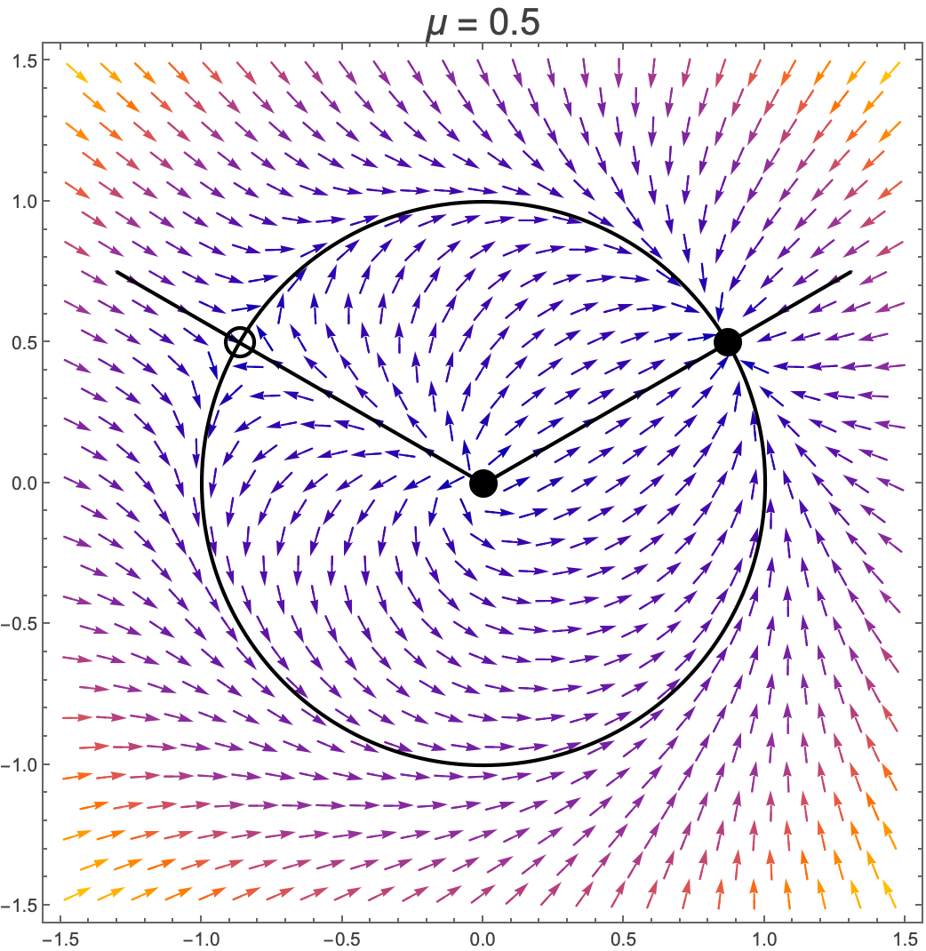
Now plotting this along with the nullclines in polar coordinates we have:

This is the case for $0\leq \mu{}<1$. For $\mu{}>1$, we just have a regular limit cycle, but for $0\leq \mu{}<1$ we see that we are going to get attracting behaviour to the rightmost fixed point and repelling from the left. This looks like

So what happens as we get to $\mu{}=1 \text{ from } $above? Well, just plotting the vector field we see:

which doesn’t look terribly interesting…however, for $\mu{} \text{ just above }$ 1, we see that while there isn’t a fixed point, there will be a point where $\mu{}-\text{ sin }\left(\theta{}\right)$ gets very very small (just never hitting zero). That means that if we are on the limit cycle, as we get close to $\theta{}=\frac{\pi{}}{2}, $$\dot{\theta{}}$ will get very very small, and so we will slow down enormously as we get to this point. This looks like:

In fact we can plot the trajectory on the unit circle as a function of time for different values of μ. Plotting $\cos\left(\theta\right)$ (the projection onto the x-axis) we get (red is 1.05, green is 1.2, blue is 1.5):

Can we calculate the period of the oscillation by integrating the differential equation:

$$ \dot{\theta{}}=\mu{}-\text{ sin }\left(\theta{}\right) $$

The period is how long θ takes to get from 0 to 2π, so we write:

$$ T={\int{}}_{0}^{2\pi{}}\frac{1}{\mu{}-\text{ sin }\left(\theta{}\right)}\mathrm{d}\theta{}=\frac{2\pi{}}{\sqrt{{\mu{}}^{2}-1}} $$

So as $\mu{}\to 1, $the period goes to infinity. This therefore is called an Infinite Period Bifurcation.

What we see from the animation (and from the equation) is that at the top of the orbit it’s very slow, but at the bottom it’s very fast. Most of the $\frac{2\pi{}}{\sqrt{{\mu{}}^{2}-1}}$time is spent up at the top of the orbit

Deep breath…we have one more limit cycle bifurcation to go, and that is a Homoclinic (or saddle-loop) Bifurcation. The ingredients needed for this are a saddle, and a limit cycle. When the limit-cycle hits the saddle, the bifurcation occurs. It’s not easy to find simple examples of this, so the following simply illustrates what happens in the case of

$$ \dot{x}=y $$$$ \dot{y}=\mu{} y+x-x^{2}+x y $$

Here I show characteristic trajectories for $\mu{}=-1, \mu{}=-0.8645 \text{ and } \mu{}=-0.8$. On the left you can see that there is a limit cycle in blue. As μ increases the limit cycle moves closer to the saddle at $\left(0,0\right)$ and as it hits the saddle, it connects with the unstable manifold and disintegrates such that trajectories which previously were attracted to the limit cycle now necessarily hit the unstable manifold moving to the bottom left.

precisely at the bifurcation point (the middle point), we get a homoclinic orbit.

In the next section we’re going to talk about coupled oscillators and periodicity, and then we will start edging closer to chaos…