Section 3.1: Saddle-nodes, transcritical and pitchfork bifurcations in two dimensions

Section 3.1: Saddle-nodes, transcritical and pitchfork bifurcations in two dimensions

We spent a lot of time last year looking at bifurcations in one dimensional systems. Remember they correspond to having some parameter in our system which we can tune, and as we do so the fixed point structure changes. Essentially it was about stable and unstable fixed points coming together and annihilating, or appearing out of thin air, or swapping stabilities. $\left(0\to 2,2\to 0,2\to 2,1\to 3 \text{ or } 3\to 1\right)$.

Now that we have moved up from one dimensional systems to two dimensional systems, presumably we are going to have a much richer structure of the way that bifurcations can happen…well, for the most part that’s not quite true, at least not when we are simply looking at fixed points bumping into each other and changing in the various ways that they could in one dimension.

For the basic types of bifurcations that we looked at before, fixed points still have to come together for a bifurcation to occur, and just because they can do so in a plane rather than on a line doesn’t make the types of behaviour possible much richer. In fact things will get more interesting only when we start to think about limit cycles, which of course can’t occur in one dimension.

Remember in a one-dimensional system a fixed point is just give by solving

$$ \dot{x}=f\left(x\right) $$

for

$$ \dot{x}=0 $$

Well, a fixed point in two dimensions, as we’ve talked about before is just given by

$$ \dot{x}=0 $$$$ \dot{y}=0 $$

If we just look at one of these on its own, then we get one of the null-clines. ie. if we look only at

$$ \dot{x}=0 $$

and leave $\dot{y}$ unconstrained, then we are looking at those trajectories where the movement is entirely in the y-direction. Similarly the other way around. So in fact if we look for the null-clines corresponding to each of the equations being zero separately, and ask where they intersect, then we can find the fixed points.

$$ \dot{x}=y $$$$ \dot{y}=x-x^{3} $$

Which has trajectories given by:

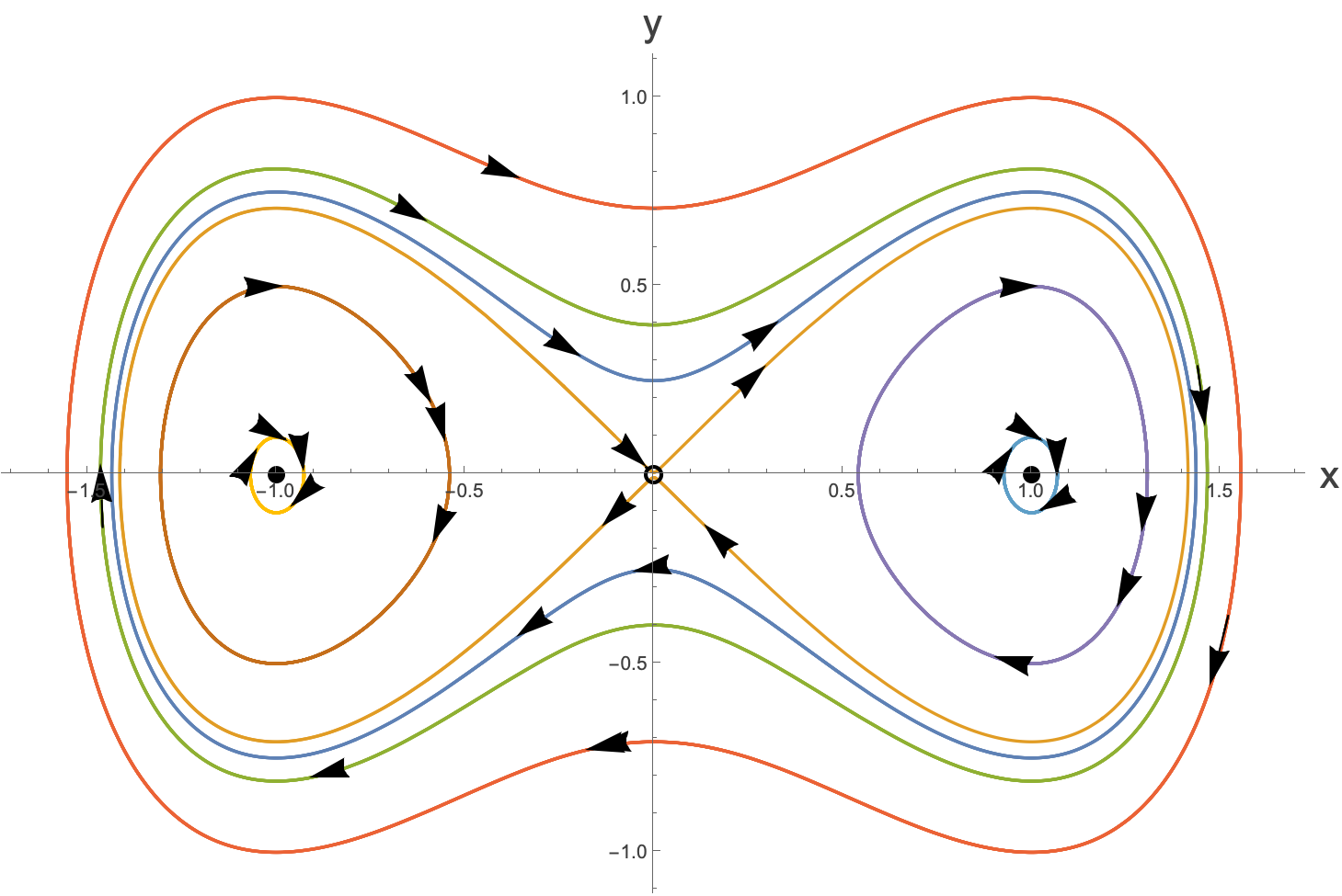
If we look at nullclines rather than trajectories, then we are asking to write down the curves corresponding to:

$$ y=0 $$

and

$$ x-x^{3}=0 $$

separately. Plotting these as dashed lines on the trajectories in the phase space we see:

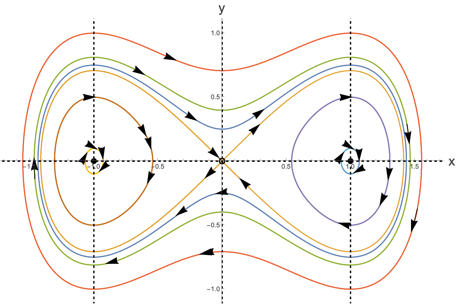
The intersections of the null-clines are the fixed points.

OK, so let’s look at a slightly different example now. Let ’s take the vector field given by:

$$ \dot{x}=-a x+y $$$$ \dot{y}=\frac{x^{2}}{1+x^{2}}-b y $$

where for now $a \text{ and } b$ are just free (but positive) parameters and we will take $x \text{ and } y$ to both be also positive.

The null-clines are given by the two separate equations:

$$ 0=-a x+y \to y=a x $$$$ 0=\frac{x^{2}}{1+x^{2}}-b y \to y=\frac{x^{2}}{b \left(1+x^{2}\right)} $$

Plotting this for a particular choice of $a$ and $b$ we have:

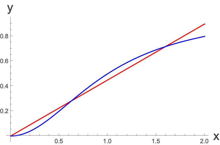
For $a=0.45 \text{ and } b=1$ we seem to have three fixed points (three points of intersection here).

From this picture it should be clear what happens as we change $a$ and $b$. They will just alter the gradients of the curves. You can see that if the red gradient gets larger here compared to the blue, two of the fixed points will come together and disappear. In fact we should be able to work out exactly when this happens.

To find the positions of the fixed points we just have to solve the null-cline equations simultaneously:

$$ y=a x \text{ and } y=\frac{x^{2}}{b \left(1+x^{2}\right)} $$$$ a x=\frac{x^{2}}{b \left(1+x^{2}\right)} \to x=0, x=\frac{1\pm{}\sqrt{1-4 a^{2} b^{2}}}{2 a b} $$

The x=0 fixed point is there independent of the values of $a$ and $b$, but the other fixed points are only there if the term inside the square root is real. Indeed those two fixed points become one when:

$$ 1-4 a^{2} b^{2}=0 \to a=\frac{1}{2b} $$

Fixing $b=1 $we have the following, with $a$ varying, and the vector field plotted over the top:

What do we see? We see two fixed points coming together as the parameter changes, and annihilating.

But why are we doing this in terms of null-clines all of a sudden? Well, let ’s think about what we have here…it’s two lines intersecting at two points. Those two points come together, and then the intersection disappears. This is actually exactly like the one-dimensional case, where we would plot the graph of

$$ \dot{x}=f\left(x\right) $$

and the fixed points would be the intersection with the x-axis. It ’s the same thing - the intersection of two curves…it ’s just that in the one-dimensional case, one of the curves is just the x-axis. Let’s look at a simple example in one dimension:

So it’s not that surprising that nothing much more interesting can happen in two-dimensions. It’s still about lines intersecting, it just so happens that rather than the $\dot{x}$=0 null-cline intersecting with the $\dot{x}$=f(x) line, it’s the $\dot{x}=0$ and $\dot{y}=0$ lines intersecting.

What we have looked at here is a saddle-node bifurcation in a two-dimensional system. Previously (in one-dimensional systems) we plotted bifurcation patterns of the position of the critical points $x_{\text{ crit }}$versus the control parameter. Here we really have a three dimensional system (if there is only a single control parameter) where we have $\left(x_{\text{ crit }},y_{\text{ crit }}\right)$ as a function of the control parameter, so it’s not as easy to plot these as in a one-dimensional system.

Let’s go back to the example above quickly. We said that there were three fixed points at

$$ x=0, x=\frac{1\pm{}\sqrt{1-4 a^{2} b^{2}}}{2 a b} $$

Clearly this is only true for certain values of $a \text{ and } b$. Indeed we can see that the critical point occurs when

$$ a_{c}=\frac{1}{2b} $$

Can we learn anything about the types of fixed points? Well, remember that we can look at the Jacobian of the system at the fixed points. The Jacobian is:

$$ A=\left(\begin{matrix} {\partial{}}_{x}f & {\partial{}}_{y}f \\ {\partial{}}_{x}g & {\partial{}}_{y}g \end{matrix}\right)=\left(\begin{matrix} -a & 1 \\ \frac{2x}{{\left(1+x^{2}\right)}^{2}} & -b \end{matrix}\right) $$

Which at the fixed points is:

$$ A_{x=0}=\left(\begin{matrix} -a & 1 \\ 0 & -b \end{matrix}\right) , A_{x=\frac{1-\sqrt{1-4 a^{2} b^{2}}}{2 a b}}=\left(\begin{matrix} -a & 1 \\ a b \left(1+\sqrt{1-4 a^{2} b^{2}}\right) & -b \end{matrix}\right), A_{x=\frac{1+\sqrt{1-4 a^{2} b^{2}}}{2 a b}}=\left(\begin{matrix} -a & 1 \\ a b \left(1-\sqrt{1-4 a^{2} b^{2}}\right) & -b \end{matrix}\right) $$

The trace of this is always negative, so depending on the sign of the determinant, you will either have a saddle, or a purely attractive node (a sink). There are no unstable spirals, for instance.

The determinant is

$$ {\Delta{}}_{x=0}=a b>0, {\Delta{}}_{x=\frac{1-\sqrt{1-4 a^{2} b^{2}}}{2 a b}}=-a b\sqrt{1-4 a^{2} b^{2}}, {\Delta{}}_{x=\frac{1+\sqrt{1-4 a^{2} b^{2}}}{2 a b}}=a b\sqrt{1-4 a^{2} b^{2}} $$

So the $x=0 \text{ fixed }$ point appears either to be a stable node or stable spiral. Reminding ourselves of our favourite diagram we have:

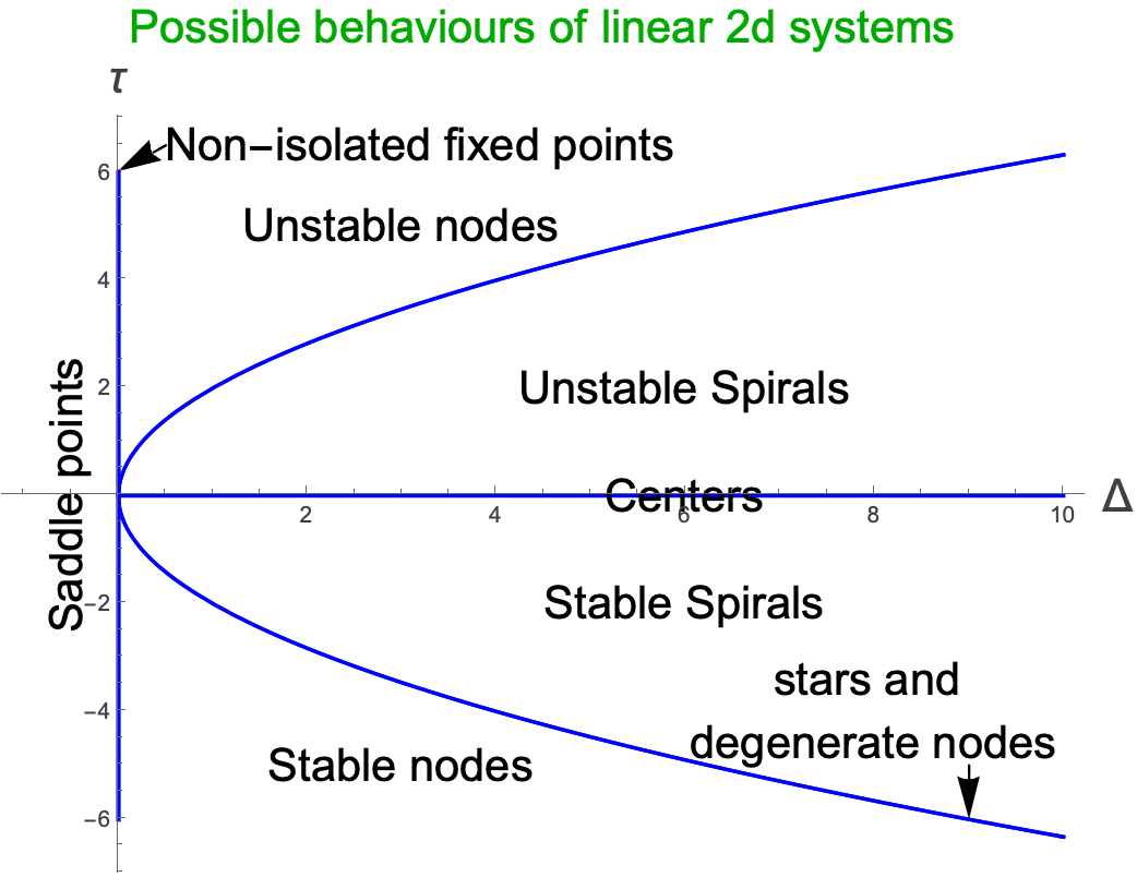
So for a stable spiral, we would need to have τ negative, which we do, and we would have to have $\tau{}>-\sqrt{4 \Delta{}} \to {\tau{}}^{2}-4\Delta{}<0$, ie.

$$ {\left(-a-b\right)}^{2}-4 a b<0 \text{ implying } {\left(a-b\right)}^{2}<0 $$

However, there is no value of $a$ and $b$ for which this is true, so we always have a stable node at $x=0.$

The next fixed point along in increasing $x$ is a saddle point (both τ and Δ negative), and then the last one is either a stable node or a stable spiral. Again, for it to be a stable spiral we would need:

$$ {\left(-a-b\right)}^{2}-4 a b\sqrt{1-4 a^{2} b^{2}}<0 $$

but the left hand side is actually greater than ${\left(a-b\right)}^{2}$ so again it can never be negative and this is a stable node.

We see, as we have seen before, that in the case where there are three fixed points, the middle one being a saddle, there is a stable manifold which separates the space into attractors for the two stable fixed points:

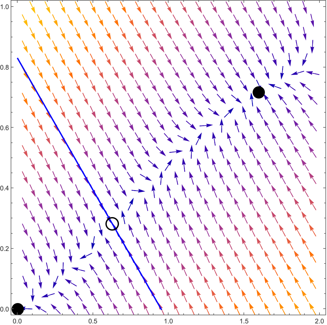
To the bottom left of the blue line everything flows to the fixed point at 0. To the top right of the blue line everything flows to the non-zero fixed point.

OK, so we’ve spent a lot of time now looking at saddle-node bifurcations. How about the other types that we see in one-dimension. Well, I ’m going to leave it as an exercise for you to explore the following bifurcations:

$$ \dot{x}=\mu{} x-x^{2}, \dot{y}=-y $$$$ \dot{x}=\mu{} x-x^{3}, \dot{y}=-y $$$$ \dot{x}=\mu{} x+x^{3}, \dot{y}=-y $$

While these examples are decoupled, and so in some sense even more similar to the one-dimensional cases we’ve already seen, you should see that we could rotate the plane and create non-linear combinations of $x \text{ and } y$ such that the examples are less trivial, but still qualitatively the same.

Also explore the example

$$ \dot{x}=\mu{} x+y+\text{ sin } x, \dot{y}=x-y $$