Section 2.6: Weakly nonlinear oscillators
Section 2.6: Weakly nonlinear oscillators
Not the Van der Pol oscillator again, I hear you cry!! Yep, I ’m afraid so…but this time in a different limit. Not the limit of very strong nonlinearities, but the opposite limit, where it ’s very close to linear:
$$ \ddot{x}+\epsilon{} \left(x^{2}-1\right)\dot{x} +x=0 $$where now ε is going to be treated as a small value.
In fact we are going to be studying more general systems than this. We are going to me looking at systems of the form
$$ \ddot{x}+x+\epsilon{} h\left(x,\dot{x} \right)=0 $$where $h\left(x,\dot{x} \right)$ is some smooth function, and $0\leq \epsilon{}\ll 1$.
We’re going to ask, in the same way that we did when this term was very large, what can we learn about such a system with this approximation?
In fact the answer seems kind of obvious…I hope. For the Van der Pol oscillator, if we treat the term proportional to ε as being small, and we start at some small value of $x, \text{ then we } \text{ are going } $to be approximately moving according to
$$ \ddot{x}=-x $$which gives circular motion, but we will have a term of the form:
$$ \ddot{x}=-x-\epsilon{} \left(\text{ small and } \text{ negative }\right)\dot{x} $$which says that we will have an additional contribution of the acceleration in the direction of motion, which drives us slightly out from circular motion. As we get closer and closer to $x=1, \text{ this small } \text{ additional term } \text{ becomes }$ even smaller, and so we get a better and better approximation to
$$ \ddot{x}=-x $$as we approach $x=1$. For ε=0.1, we have:
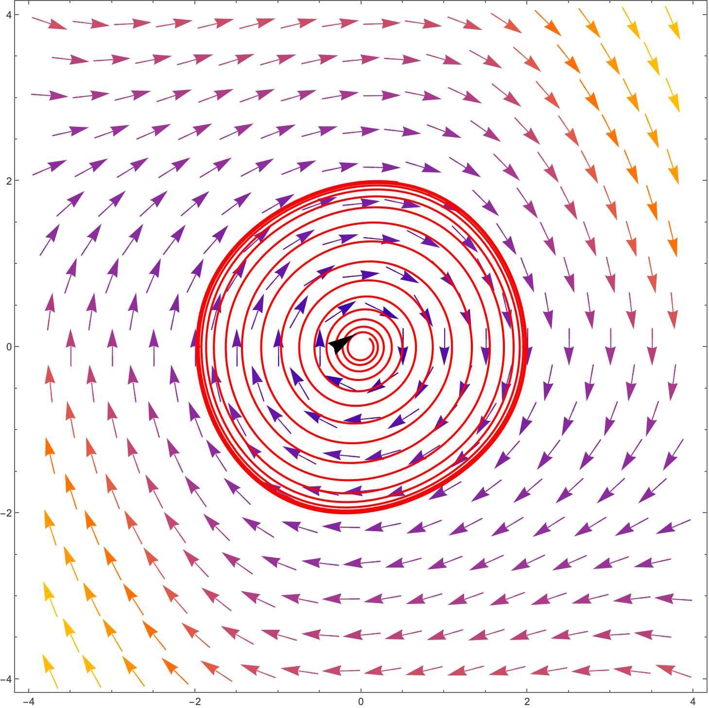
We’ve gone from the complicated motion of the Van Der Pol oscillator, to a pretty simple version which is more or less circular motion with a slight movement out for $x<1$ and a slight movement in for $x>1$.
The same thing happens with the so-called Duffing equation, given by:
$$ \ddot{x}+\delta{} \dot{x}+\alpha{} x+\beta{} x^{3}=\gamma{} \text{ cos }\left(\omega{} t\right) $$This is of course a three dimensional system, but taking $\alpha{}=1, \delta{}=\gamma{}=0$, we have:
$$ \ddot{x}+x+\beta{} x^{3}=0 $$which for $\beta{}=0.1 \text{ on the } \text{ left and } \beta{}=2 \text{ on the } \text{ right }$ look like:
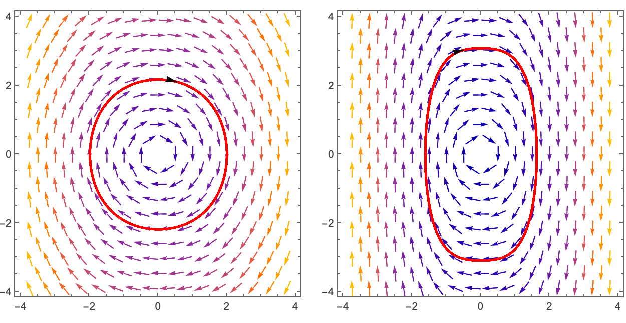
The Duffing equation is itself very interesting, and we may discuss it more later.
Exercise: By taking the Duffing equation and multiplying by $\dot{x}$, and integrating, find a conserved quantity. Given that there is a fixed point at $\left(x,\dot{x}\right)=\left(0,0\right)$, what does this tell you? Plot the energy surface.
Anyway, we’re going on tangents here, let’s get back to business…
As you get back to business, make sure that you have a pen and a pad of paper with you. Write all of what follows down and make sure that you can understand every step of the mathematics!
So, given an equation of the form:
$$ \ddot{x}+x+\epsilon{} h\left(x,\dot{x} \right)=0 $$You might think that you could perform a perturbative analysis. This is often the case when you have a small parameter in the system. You set up the solution as a series expansion in the small parameter, plug in the series to the equation and solve order by order. Seems not implausible, so let ’s give it a go.
Let’s look at the particular example:
$$ \ddot{x}+x+2\epsilon{} \dot{x} =0 $$A series solution would look like:
$$ x\left(t\right)=x_{0}\left(t\right)+\epsilon{} x_{1}\left(t\right)+{\epsilon{}}^{2}x_{2}\left(t\right)+... $$Sometimes you will see the left hand side written as $x\left(t,\epsilon{}\right), \text{ but we } $will miss out the ε here. Let’s see if we can find these different $x_{k}\left(t\right)$ for a given initial condition:
$$ x\left(0\right)=0, \dot{x}\left(0\right)=1 $$This also means that we can set $x_{0}\left(0\right)=0, x_{0}'\left(0\right)=1$ and all other $x_{k}\left(0\right), x_{k}'\left(0\right)=0$. Why? Because the ε should not affect the first order term, so it can’t be ε dependent, therefore it must give us the initial condition. Note that we’re using ‘ rather than dots here for the time derivative. It’s just a notation convention, but you can use either.
Actually, the equation can be solved exactly to get:
But here we want to presume that we don’t know the analytical solution and find an approximation. Plugging in our perturbative solution to the equation we get:
$$ \frac{d^{2}}{d t^{2}}\left(x_{0}\left(t\right)+\epsilon{} x_{1}\left(t\right)+{\epsilon{}}^{2}x_{2}\left(t\right)+...\right)+\left(x_{0}\left(t\right)+\epsilon{} x_{1}\left(t\right)+{\epsilon{}}^{2}x_{2}\left(t\right)+...\right)+2\epsilon{} \frac{d}{d t}\left(x_{0}\left(t\right)+\epsilon{} x_{1}\left(t\right)+{\epsilon{}}^{2}x_{2}\left(t\right)+...\right)=0 $$The idea at this point is that you collect together terms at each order in $\epsilon{}$:
$$ \left(x_{0}''\left(t\right)+x_{0}\left(t\right)\right)+\epsilon{} \left(x_{1}''\left(t\right)+x_{1}\left(t\right)+2x_{0}'\left(t\right)\right)+{\epsilon{}}^{2}\left(x_{2}''\left(t\right)+x_{2}\left(t\right)+2x_{1}'\left(t\right)\right)+O\left({\epsilon{}}^{3}\right)=0 $$ok, so now we state that because the $x_{k}\left(t\right)$ solutions themselves don’t depend on ε, we should be able to solve order by order:
$$ \left(x_{0}''\left(t\right)+x_{0}\left(t\right)\right)=0 $$$$ \left(x_{1}''\left(t\right)+x_{1}\left(t\right)+2x_{0}'\left(t\right)\right)=0 $$$$ \left(x_{2}''\left(t\right)+x_{2}\left(t\right)+2x_{1}'\left(t\right)\right)=0 $$So if we solve the $x_{0}\left(t\right)$ we can then plug it into the second equation and solve for $x_{1}\left(t\right) \text{ etc }.$
The first equation has solution
$$ x_{0}\left(t\right)=c_{1}\text{ cos }\left(t\right)+c_{2}\text{ sin }\left(t\right) $$where $c_{2}=1 \text{ and } c_{1}=0 $by the initial conditions. Now going to the second equation we have:
$$ x_{1}''\left(t\right)+x_{1}\left(t\right)=-2\text{ cos }\left(t\right) $$hmmm…but this is a resonant driving force. We can solve this and it gives us:
$$ x_{1}\left(t\right)=-t \text{ sin }\left(t\right) $$But now we have a problem. We have said that $\epsilon{}$ is small, but in fact what we really need is that $\epsilon{} x_{1}\left(t\right) \text{ is small } \text{ compared }$ to $x_{0}\left(t\right)$, but now we have this $t \text{ term }$, so for large times, this second term is clearly not going to be smaller than the first term. In fact the second term is going to start to dominate when
$$ t \epsilon{}\gtrsim{}1 $$because just going up to this second term our series expansion now looks like:
$$ x\left(t\right)=\text{ sin }\left(t\right)-\epsilon{} t \text{ sin }\left(t\right)+{\epsilon{}}^{2}x_{2}\left(t\right)+... $$So perhaps we can trust this series solution for small times, but not for times greater than of order $\frac{1}{\epsilon{}}.$
Plotting the true solution, and the first two terms of the series solution we see the following, for $\epsilon{}=0.1:$
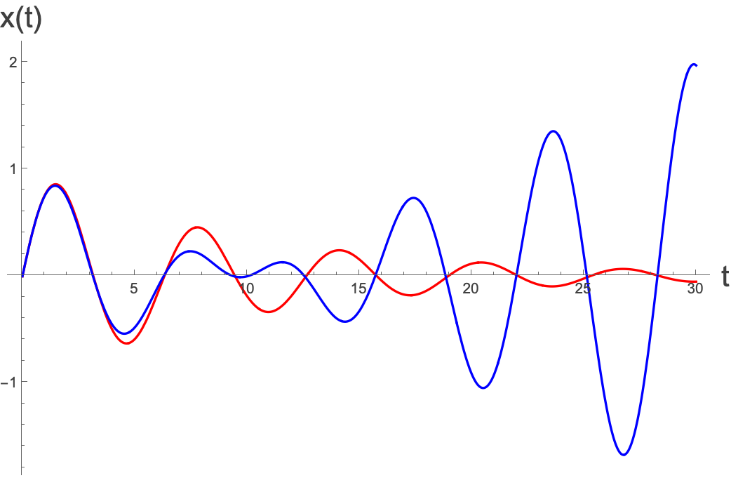
Where the red is the true solution, and the blue is the series solution, which is a reasonable approximation up to around t=4, and then after that it diverges a lot.
In fact we see that while the fast oscillations seem to be in ‘rhythm’ between the two functions, over the longer timescale, the true solution exponentially converges, whereas the series solution diverges.
We say that the short timescale behaviours (the oscillations) agree, but the longer timescale behaviours disagree. The reason for this is quite simple. If we take the true solution, it is given by:
$$ x\left(t\right)=e^{-\epsilon{} t }\frac{\text{ sin }\left(\sqrt{1-{\epsilon{}}^{2}}t\right)}{\sqrt{1-{\epsilon{}}^{2}}} $$There is a fast timescale behaviour given by the sinusoidal motion, and there’s an exponential decay dominated by $e^{-t \epsilon{}}$. We can say that the fast timescale is O(1), and the slow timescale is O(1/ε).
On the other hand, the timescale of the incorrect blowup is O(1).
If we perform a series expansion of this last part it is given by:
$$ e^{-\epsilon{} t }=1-\epsilon{} t+\frac{{\left(\epsilon{} t\right)}^{2}}{2}-... $$we know that this is exact, for arbitrary $\epsilon{} t$, but if $\epsilon{} t$ is large, then you need to take a very large number of terms. This is the issue that has arisen. We stopped at the second term…and that wasn ’t unreasonable, as we wanted to do this for small ε…but it’s not the size of ε that is important, it’s the size of ε $t$.
What we see here is a general phenomenon. For any weakly nonlinear oscillator, we are going to have a timescale given by the purely linear approximation, then we’re going to have another timescale dictated by $\frac{1}{\epsilon{}}.$
So can we still use a perturbative method? It turns out that we can, but we have to do a bit of a change of variables.
Pause: We have mentioned timescales a bunch of times here, but what do we really mean. Well, it all feels a bit vague and hand-wavey, but what we really mean are the characteristic time over which there is a substantial change in some aspect of a system (an oscillator, a phase, an amplitude). If you have a periodic function of the form $f\left(t\right)=\text{ sin }\left(t\right)$, and let’s say that $t $is measured in seconds, then if you look at your system at time $t=0$ and time $t=0.01$, then your system isn’t going to have changed much. By timescale here we really mean, over what minimum order of magnitude of time will we see a noticeable change. There are lots of vague notions in here. What do we mean by “noticeable change ”? Also, what do we mean by order of magnitude. We really mean here not that we care about whether it’s 1 second, or 1.1 seconds, but whether it’s 1 second, or 0.1 seconds, or 10 seconds, etc. And in this case, because the frequency is $\frac{1}{2\pi{}}$, we can say that the timescale over which things change substantially is on the order of 1 second. After 1 second, you’ve completed 1/2π of the whole oscillation. After $\frac{4}{2\pi{}} \text{ seconds you }'\text{ ve gone } \text{ from } 0$ to the maximum of the oscillation, so this is a reasonable measure for the characteristic timescale.
For the exponential part, we are really again asking over which time period are you seeing a substantial change, and here after time of order 1/ε, the term $e^{\epsilon{} t}$ has changed by a factor of $e$. Of course we could say that it had already changed a reasonable amount after $\frac{1}{2\epsilon{}}$but we are just interested in the order of magnitude, and so we just care about the relative difference in timescales. One is of order 1 and one is of order $\frac{1}{\epsilon{}}.$
Such ideas come up in dynamical systems in the real world a lot. For instance, in the brain, there are multiple timescales:
Neurons fire over timescales of $O\left({10}^{-3}s\right)$
Sensory processing and short term memory occur over timescales of $O\left({10}^{0}-{10}^{2}s\right)$
Long-term potentiation and learning occur over timescales of $O\left({10}^{1}-{10}^{4}s\right)$
Long-term memory and synaptic pruning occur over timescales of $O\left({10}^{3}-{10}^{6}s\right)$
Neuroplasticity and aging occur over timescales of $O\left({10}^{5}-{10}^{8}s\right)$
These numbers are all up for debate, and you’ll find other figures floating around, but you get the general idea. The dynamics of such a system is very complex and there is dynamics happening at the millisecond, second, minute, hour, day, month, year timescale. They also overlap, which makes modelling such processes really hard, as you can’t really deal with any one of them alone.
OK, on to the problem at hand.
The solution depends on two timescales, which we will treat as independent variables. We let $\tau{}=t$ be the fast time, and $T=\epsilon{} t $be the slow time. Now we set up our series expansion as before but now with;
$$ x\left(t\right)=x_{0}\left(\tau{},T\right)+\epsilon{} x_{1}\left(\tau{},T\right)+{\epsilon{}}^{2}x_{2}\left(\tau{},T\right)+... $$Now the total derivative in t gives us:
$$ \frac{d}{d t}=\frac{\partial{}}{\partial{} \tau{}}+\frac{\partial{} T}{\partial{} t}\frac{\partial{}}{\partial{} T}=\frac{\partial{}}{\partial{} \tau{}}+\epsilon{}\frac{\partial{}}{\partial{} T} $$Plugging the series expansion into the equation using the new variables gives:
$$ \left(\frac{\partial{}}{\partial{} \tau{}}+\epsilon{}\frac{\partial{}}{\partial{} T}\right)\left(\frac{\partial{}}{\partial{} \tau{}}+\epsilon{}\frac{\partial{}}{\partial{} T}\right)\left(x_{0}\left(\tau{},T\right)+\epsilon{} x_{1}\left(\tau{},T\right)+{\epsilon{}}^{2}x_{2}\left(\tau{},T\right)\right)+\left(x_{0}\left(\tau{},T\right)+\epsilon{} x_{1}\left(\tau{},T\right)+{\epsilon{}}^{2}x_{2}\left(\tau{},T\right)\right)+2\epsilon{} \left(\frac{\partial{}}{\partial{} \tau{}}+\epsilon{}\frac{\partial{}}{\partial{} T}\right)\left(x_{0}\left(\tau{},T\right)+\epsilon{} x_{1}\left(\tau{},T\right)+{\epsilon{}}^{2}x_{2}\left(\tau{},T\right)\right)=0 $$Taking the zeroth order terms we have:
$$ \frac{{\partial{}}^{2}}{\partial{} {\tau{}}^{2}}x_{0}\left(\tau{},T\right)+x_{0}\left(\tau{},T\right)=0 $$Which has solutions
$$ x_{0}\left(\tau{},T\right)=A\left(T\right)\text{ cos }\left(\tau{}\right)+B\left(T\right) \text{ sin }\left(\tau{}\right) $$Where the functions $A \text{ and } B $are not fixed. This sounds kind of ridiculous! But actually if we now go to the next order in ε, we have the equation:
$$ \frac{{\partial{}}^{2}}{\partial{} {\tau{}}^{2}}x_{1}\left(\tau{},T\right)+2\frac{\partial{}}{\partial{} T}\frac{\partial{}}{\partial{} \tau{}}x_{0}\left(\tau{},T\right)+ x_{1}\left(\tau{},T\right)+2\frac{\partial{}}{\partial{} \tau{}}x_{0}\left(\tau{},T\right)=0 $$and now we can plug our solution above in to get:
$$ \frac{{\partial{}}^{2}}{\partial{} {\tau{}}^{2}}x_{1}\left(\tau{},T\right)+2\frac{\partial{}}{\partial{} T}\frac{\partial{}}{\partial{} \tau{}}\left(A\left(T\right)\text{ cos }\left(\tau{}\right)+B\left(T\right) \text{ sin }\left(\tau{}\right)\right)+ x_{1}\left(\tau{},T\right)+2\frac{\partial{}}{\partial{} \tau{}}\left(A\left(T\right)\text{ cos }\left(\tau{}\right)+B\left(T\right) \text{ sin }\left(\tau{}\right)\right)=0 $$$$ \frac{{\partial{}}^{2}}{\partial{} {\tau{}}^{2}}x_{1}\left(\tau{},T\right)+2\left(-A'\left(T\right)\text{ sin }\left(\tau{}\right)+B'\left(T\right) \text{ cos }\left(\tau{}\right)\right)+ x_{1}\left(\tau{},T\right)+2\left(-A\left(T\right)\text{ sin }\left(\tau{}\right)+B\left(T\right) \text{ cos }\left(\tau{}\right)\right)=0 $$which we can rewrite as:
$$ \frac{{\partial{}}^{2}}{\partial{} {\tau{}}^{2}}x_{1}\left(\tau{},T\right)+ x_{1}\left(\tau{},T\right)=-2\text{ sin }\left(\tau{}\right)\left(A\left(T\right)+A'\left(T\right)\right)+2\text{ cos }\left(\tau{}\right)\left(B\left(T\right)+B'\left(T\right)\right) $$How could we ensure that we don’t have a resonant driving force here? Well, we can do this by setting:
$$ \left(A\left(T\right)+A'\left(T\right)\right)=0 $$$$ \left(B\left(T\right)+B'\left(T\right)\right)=0 $$which means that:
$$ A\left(T\right)=A_{0}e^{-T} $$$$ B\left(T\right)=B_{0}e^{-T} $$so our $x_{0}\left(\tau{},T\right) $solution is:
$$ x_{0}\left(\tau{},T\right)=A_{0}e^{-T}\text{ cos }\left(\tau{}\right)+B_{0}e^{-T} \text{ sin }\left(\tau{}\right) $$Why did we say that there can’t be a resonant driving force? This is a bit subtle. If there was a driving force with timescale τ, we would end up with something where the τ would be not just the short-term time-scale but also the long-term timescale, which we know can’t be the case. The long-term dynamics is driven by T, not τ, so we can ’t have a driving force which makes the system explode on short time-scales.
We have to be a little careful to find our constant to match the initial conditions. Our initial conditions are:
$$ x\left(0\right)=0, \dot{x}\left(0\right)=1 $$The first of these says that:
$$ x_{0}\left(0,0\right)+\epsilon{} x_{1}\left(0,0\right)+{\epsilon{}}^{2}x_{2}\left(0,0\right)+...=0 $$We want to solve this for general small ε, which means that we must have
$$ x_{0}\left(0,0\right)=0 $$For the second condition, we have to be a bit careful and write
$$ \dot{x}\left(0\right)=\left(\frac{\partial{}}{\partial{} \tau{}}+\epsilon{}\frac{\partial{}}{\partial{} T}\right)\left(x_{0}\left(\tau{},T\right)+\epsilon{} x_{1}\left(\tau{},T\right)+{\epsilon{}}^{2}x_{2}\left(\tau{},T\right)+...\right)|_{\tau{}=0,T=0}=1 $$which has zeroth order term:
$$ \left(\frac{\partial{}}{\partial{} \tau{}}\right)\left(x_{0}\left(\tau{},T\right)\right)|_{\tau{}=0,T=0}=1 $$The reason we had to be careful here was because now there are two time-variables, so we have to be sure of what the derivative condition is with respect to.
Applying these two conditions gives:
$$ x_{0}\left(0,0\right)=A_{0}e^{-0}\text{ cos }\left(0\right)+B_{0}e^{-0} \text{ sin }\left(0\right)=A_{0}=0 $$$$ \left(\frac{\partial{}}{\partial{} \tau{}}\right)\left(x_{0}\left(\tau{},T\right)\right)|_{\tau{}=0,T=0}=-A_{0}e^{-T}\text{ sin }\left(\tau{}\right)+B_{0}e^{-T} \text{ cos }\left(\tau{}\right)|_{\tau{}=0,T=0}=B_{0}e^{-0} \text{ cos }\left(0\right)=B_{0}=1 $$So $A_{0}=0$, $B_{0}=1$ and we have
$$ x_{0}\left(\tau{},T\right)=e^{-T} \text{ sin }\left(\tau{}\right)=e^{-t \epsilon{} }\text{ sin }\left(t\right) $$This is a very good approximation to the true solution, but doesn ’t take into account a THIRD timescale which is related to the $\sqrt{1-{\epsilon{}}^{2}} \text{ term }$…but that can be left for another day…
Actually, let’s just think about the corrections. We know that the true answer is:
$$ x\left(t\right)=e^{-\epsilon{} t }\frac{\text{ sin }\left(\sqrt{1-{\epsilon{}}^{2}}t\right)}{\sqrt{1-{\epsilon{}}^{2}}} $$Let’s expand the non-exponential term in ε to see where we are going wrong:
$$ x\left(t\right)=e^{-\epsilon{} t }\left(\text{ sin }\left(t\right)+\frac{1}{2} \left(-t \text{ cos }\left(t\right)+\text{ sin }\left(t\right)\right) {\epsilon{}}^{2}\right) $$So we see that the error is:
$$ \text{ error }\left(t\right)=\frac{e^{-\epsilon{} t }}{2}\left(\text{ sin }\left(t\right)-t \text{ cos }\left(t\right)\right){\epsilon{}}^{2} $$Which is of order $1/{\epsilon{}}^{2}$.
Exercise: Now do the same thing with the Van der Pol oscillator.
In general…
Can we now come up with some methods based on the above “two-timing” method that work for general weakly nonlinear oscillations? Let’s see…
We are looking at:
$$ \ddot{x}+x+\epsilon{} h\left(x,\dot{x} \right)=0 $$and again we will define $\tau{}=t, T=t \epsilon{}, \text{ which }$ gives us:
$$ \left(\frac{\partial{}}{\partial{} \tau{}}+\epsilon{}\frac{\partial{}}{\partial{} T}\right)\left(\frac{\partial{}}{\partial{} \tau{}}+\epsilon{}\frac{\partial{}}{\partial{} T}\right)x\left(\tau{},T\right)+x\left(\tau{},T\right)+\epsilon{} h\left(x,\dot{x} \right) =0 $$which we can write more compactly as:
$$ \left({\partial{}}_{\tau{}\tau{}}+2\epsilon{} {\partial{}}_{\tau{} T}+{\epsilon{}}^{2}{\partial{}}_{TT}\right)x+x+\epsilon{} h =0 $$subbing in the series expansion
$$ x\left(t\right)=x_{0}\left(\tau{},T\right)+\epsilon{} x_{1}\left(\tau{},T\right)+{\epsilon{}}^{2}x_{2}\left(\tau{},T\right)+... $$again we take order by order to give:
$$ \\{\partial{}}_{\tau{}\tau{}}x_{1}\left(\tau{},T\right)+x_{1}\left(\tau{},T\right)=-2 {\partial{}}_{\tau{} T}x_{0}\left(\tau{},T\right)-h $$where remember $h=h\left(x, \dot{x} \right)=h\left(x\left(\tau{}, T\right),\left({\partial{}}_{\tau{}}+\epsilon{} {\partial{}}_{T}\right) x\left(\tau{}, T\right)\right)$ which to zeroth order in ε is $h\left(x_{0}\left(\tau{},T\right),{\partial{}}_{\tau{}}x_{0}\left(\tau{},T\right)\right)$. So we have
$$ \\{\partial{}}_{\tau{}\tau{}}x_{1}\left(\tau{},T\right)+x_{1}\left(\tau{},T\right)=-2 {\partial{}}_{\tau{} T}x_{0}-h\left(x_{0}\left(\tau{},T\right),{\partial{}}_{\tau{}}x_{0}\left(\tau{},T\right)\right) $$we can write the solution to the first equation as the sin+cos combination, or we can write it as
$$ x_{0}\left(\tau{},T\right)=r\left(T\right)\text{ cos }\left(\tau{}+\phi{}\left(T\right)\right) $$(show that they are equivalent)
plugging this into the second equation we have:
$$ \\{\partial{}}_{\tau{}\tau{}}x_{1}\left(\tau{},T\right)+x_{1}\left(\tau{},T\right)=-2 {\partial{}}_{\tau{} T}r\left(T\right)\text{ cos }\left(\tau{}+\phi{}\left(T\right)\right)-h\left(r\left(T\right)\text{ cos }\left(\tau{}+\phi{}\left(T\right)\right),{\partial{}}_{\tau{}}r\left(T\right)\text{ cos }\left(\tau{}+\phi{}\left(T\right)\right)\right) $$which is:
$$ \\{\partial{}}_{\tau{}\tau{}}x_{1}\left(\tau{},T\right)+x_{1}\left(\tau{},T\right)=2 \left(r'\left(T\right)\text{ sin }\left(\tau{}+\phi{}\left(T\right)\right)+r\left(T\right)\phi{}'\left(T\right)\text{ cos }\left(\tau{}+\phi{}\left(T\right)\right)\right)-h\left(r\left(T\right)\text{ cos }\left(\tau{}+\phi{}\left(T\right)\right),-r\left(T\right)\text{ sin }\left(\tau{}+\phi{}\left(T\right)\right)\right) $$We don’t want any driving terms on the right hand side, so there can’t be any terms proportional to sin(τ+φ(T)) or cos(τ+φ(T)).
For the first two terms that seems pretty easy…but for the h term…how do we pull out the terms proportional to sin and cos? Let’s just simplify notation a little bit here first. We’ll remember all the functional dependencies and write the right hand side as:
$$ \\2 \left(r'\text{ sin }\left(\tau{}+\phi{}\right)+r \phi{}'\text{ cos }\left(\tau{}+\phi{}\right)\right)-h\left(r \text{ cos }\left(\tau{}+\phi{} \right),-r \text{ sin }\left(\tau{}+\phi{} \right)\right) $$and in fact we can also let τ+φ = θ to give
$$ \\2 r'\text{ sin }\left(\theta{}\right)+2r \phi{}'\text{ cos }\left(\theta{}\right)-h\left(r \text{ cos }\left(\theta{}\right),-r \text{ sin }\left(\theta{}\right)\right) $$So $h \text{ is } a \text{ periodic } $function of θ…now we get our Fourier hats on, because we know that a function which is periodic in θ can be written as:
$$ \\h\left(r \text{ cos }\left(\theta{}\right),-r \text{ sin }\left(\theta{}\right)\right)=\underset{k=0}{\overset{\infty{}}{\sum{}}}a_{k}\text{ cos }\left(k \theta{}\right)+\underset{k=1}{\overset{\infty{}}{\sum{}}}b_{k}\text{ sin }\left(k \theta{}\right) $$where the $b_{0} \text{ term }$ doesn’t appear as sin(0)=0. Here the $a_{k} \text{ and } b_{k} \text{ will be } \text{ functions of } r\left(T\right)$, but we can worry about that later.
To calculate the Fourier coefficients, you need to integrate h:
$$ \\a_{0}=\frac{1}{2\pi{}}{\int{}}_{0}^{2\pi{}}h\left(r \text{ cos }\left(\theta{}\right),-r \text{ sin }\left(\theta{}\right)\right)\mathrm{d}\theta{} $$$$ a_{k}=\frac{1}{\pi{}}{\int{}}_{0}^{2\pi{}}h\left(r \text{ cos }\left(\theta{}\right),-r \text{ sin }\left(\theta{}\right)\right)\text{ cos } \left(k \theta{}\right)\mathrm{d}\theta{}, k\geq 1 $$$$ b_{k}=\frac{1}{\pi{}}{\int{}}_{0}^{2\pi{}}h\left(r \text{ cos }\left(\theta{}\right),-r \text{ sin }\left(\theta{}\right)\right)\text{ sin } \left(k \theta{}\right)\mathrm{d}\theta{}, k\geq 1 $$This looks horrendous, but in fact when we look at a concrete example it will all become clear.
Now looking at the right hand side again we have:
$$ \\2 r'\text{ sin }\left(\theta{}\right)+2r \phi{}'\text{ cos }\left(\theta{}\right)-\underset{k=0}{\overset{\infty{}}{\sum{}}}a_{k}\text{ cos }\left(k \theta{}\right)-\underset{k=1}{\overset{\infty{}}{\sum{}}}b_{k}\text{ sin }\left(k \theta{}\right) $$The only contribution proportional to $\sin\left(\theta\right), \cos\left(\theta\right)$ (see below regarding why we don’t care about the higher order $\text{ sin }\left(k \theta{}\right) \text{ and cos }\left(k \theta{}\right)$) is:
$$ \\2 r'\text{ sin }\left(\theta{}\right)+2r \phi{}'\text{ cos }\left(\theta{}\right)-a_{1}\text{ cos }\left(\theta{}\right)-b_{1}\text{ sin }\left(\theta{}\right)=\text{ sin }\left(\theta{}\right)\left(2r'-b_{1}\right)+\text{ cos }\left(\theta{}\right)\left(2r \phi{}'-a_{1}\right) $$which must vanish, so we must have
$$ \\r'=\frac{b_{1}}{2} $$$$ r \phi{}'=\frac{a_{1}}{2} $$Which says that:
$$ \\r'=\frac{1}{2\pi{}}{\int{}}_{0}^{2\pi{}}h\left(r \text{ cos }\left(\theta{}\right),-r \text{ sin }\left(\theta{}\right)\right)\text{ sin } \left(\theta{}\right)\mathrm{d}\theta{} $$$$ r \phi{}'=\frac{1}{2\pi{}}{\int{}}_{0}^{2\pi{}}h\left(r \text{ cos }\left(\theta{}\right),-r \text{ sin }\left(\theta{}\right)\right)\text{ cos } \left(\theta{}\right)\mathrm{d}\theta{} $$which is enough information to give us our unknown functions which can then be plugged back into
$$ x_{0}\left(\tau{},T\right)=r\left(T\right)\text{ cos }\left(\tau{}+\phi{}\left(T\right)\right) $$Let’s try this for the Van der Pol oscillator:
$$ \ddot{x}+\epsilon{} \left(x^{2}-1\right)\dot{x} +x=0 $$this means that $h\left(x,\dot{x} \right)=\left(x^{2}-1\right)\dot{x} $and therefore
$$ h\left(r \text{ cos }\left(\theta{}\right),-r \text{ sin }\left(\theta{}\right)\right)=\left(r^{2}{\text{ cos }}^{2}\theta{}-1\right)\left(-r \text{ sin } \theta{}\right) $$So plugging this into the above:
$$ \\r'=\frac{1}{2\pi{}}{\int{}}_{0}^{2\pi{}}\left(r^{2}{\text{ cos }}^{2}\theta{}-1\right)\left(-r \text{ sin } \theta{}\right)\text{ sin } \left(\theta{}\right)\mathrm{d}\theta{} $$$$ r \phi{}'=\frac{1}{2\pi{}}{\int{}}_{0}^{2\pi{}}\left(r^{2}{\text{ cos }}^{2}\theta{}-1\right)\left(-r \text{ sin } \theta{}\right)\text{ cos } \left(\theta{}\right)\mathrm{d}\theta{} $$Taking the first of these we can write the integral as:
$$ \\\frac{r}{2\pi{}}{\int{}}_{0}^{2\pi{}}{\text{ sin }}^{2}\theta{}\mathrm{d}\theta{}-\frac{r^{3}}{2\pi{}}{\int{}}_{0}^{2\pi{}}{\text{ cos }}^{2}\theta{} {\text{ sin }}^{2}\theta{}\mathrm{d}\theta{} $$These integrals of the form:
$$ \\\frac{1}{2\pi{}}{\int{}}_{0}^{2\pi{}}f\left(\theta{}\right)\mathrm{d}\theta{} $$Are the average of $f\left(\theta{}\right) \text{ over } $one wavelength which gives:
$$ \\\frac{r}{2}-\frac{r^{3}}{8} $$So we have
$$ \\r'=\frac{r}{2}-\frac{r^{3}}{8} $$Remember that $r=r\left(T\right)$. We can integrate this to get:
$$ \\r=\frac{\sqrt{k}2 e^{T/2}}{\sqrt{k e^{T}+1}} $$and for the second equation we have:
$$ r \phi{}'=\frac{1}{2\pi{}}{\int{}}_{0}^{2\pi{}}\left(r^{2}{\text{ cos }}^{2}\theta{}-1\right)\left(-r \text{ sin } \theta{}\right)\text{ cos } \left(\theta{}\right)\mathrm{d}\theta{}=0, \text{ which implies } \text{ that } \phi{}=\text{ constant }. $$with initial condition $x\left(0\right)=1, x'\left(0\right)=0$, we have, for the first of these:
$$ x_{0}\left(0,0\right)=r\left(0\right)\text{ cos }\left(0+\phi{}\left(0\right)\right)=1 $$and for the second
$$ \left(\frac{\partial{}}{\partial{} \tau{}}\right)\left(r\left(T\right)\text{ cos }\left(\tau{}+\phi{}\left(T\right)\right)\right)|_{\tau{}=0,T=0}=r\left(0\right)\text{ sin }\left(0+\phi{}\left(0\right)\right)=0 $$so squaring each of these equations and adding them gives us:
$$ {r\left(0\right)}^{2}{\text{ cos }}^{2}\left(\phi{}\left(0\right)\right)+{r\left(0\right)}^{2}{\text{ sin }}^{2}\left(\phi{}\left(0\right)\right)=1 $$meaning that
$$ r\left(0\right)=1 $$taking the positive root. This fixes:
$$ \\r=\frac{2 }{\sqrt{1+3e^{-T}}} $$and finally
$$ \text{ cos }\left(\phi{}\left(0\right)\right)=1 $$$$ \phi{}\left(0\right)=0 $$which because we know that φ is constant, means that it’s identically zero. Now, the overall solution is:
$$ x_{0}\left(\tau{},T\right)=\frac{2 }{\sqrt{1+3e^{-T}}}\text{ cos }\left(\tau{}\right) $$and so:
$$ x\left(\tau{},T\right)=\frac{2 }{\sqrt{1+3e^{-T}}}\text{ cos }\left(\tau{}\right)+O\left(\epsilon{}\right) $$converting back into t and ε we have:
$$ x\left(t\right)=\frac{2 }{\sqrt{1+3e^{-t \epsilon{}}}}\text{ cos }\left(t\right)+O\left(\epsilon{}\right) $$One thing that you might be a bit confused about is why we don ’t care about having contributions of $\sin$ and $\cos\left(k\theta\right)$ for $k>1$ on the right hand side.
The point is that if we have a system of the form
$$ \ddot{x} +x=\text{ cos }\left(t\right) $$then the period of the system
$$ \ddot{x} +x=0 $$is the same as the period of the system $\cos\left(t\right)$. So the two will synch up and you will get exponential growth on timescales of O(1). Imagine having a swing which swings every second, and then push on that in synch with it. You will always be adding to the oscillations and the swing will quickly diverge from any small oscillation you may have started with.
On the other hand if you force it with twice the frequency, then half the time you will be pushing in the direction that it’s going, and half the time you will be pushing it against its motion. Looking at plots of
$$ \ddot{x} +x=\text{ cos }\left(t\right) \text{ and } \ddot{x} +x=\text{ cos }\left(2t\right) $$we see:
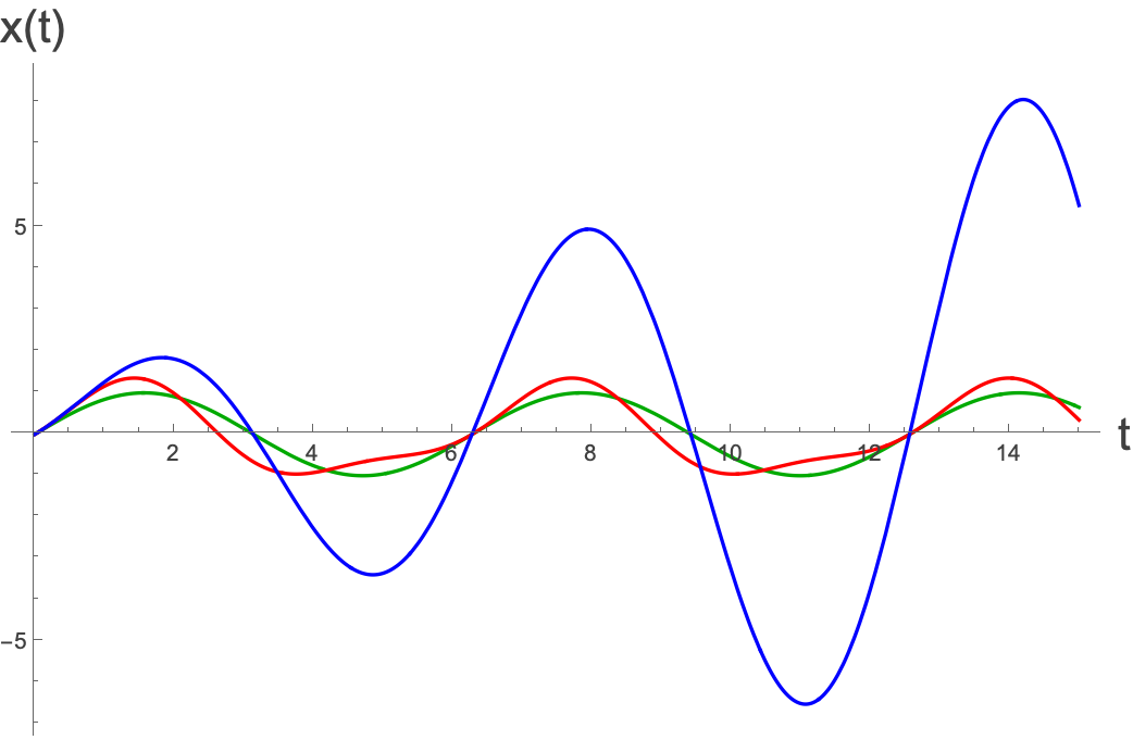
where the blue line is being driven at the natural frequency of the system, and the red line is being driven at twice the natural frequency and is thus only perturbed slightly away from the natural rhythm (in green).
How could we have known from the start that $\epsilon t$ was the right combination?
Could we have known that the right second time quantity was $\epsilon{} t$? Let’s look again at the original equation:
$$ \ddot{x}+x+2\epsilon{} \dot{x} =0 $$Let’s write it out like:
$$ \frac{d^{2}x}{d t^{2}}+x+2\epsilon{} \frac{dx}{\text{ dt }}=0 $$If we let $\epsilon{} t=T$ and $\tau{}=t$, then we can get rid of the ε completely by writing:
$$ \frac{d^{2}x}{d {\tau{}}^{2}}+x+2 \frac{dx}{\text{ dT }}=0 $$This is how we could see from the start that $\epsilon{} t$ would be the right second time variable.