Section 2.5: Relaxation oscillations

Section 2.5: Relaxation oscillations

In this section and the next we are going to look at systems where particular parameters can be taken as large and ask if we can get some understanding beyond the fact that there are simply closed cycles. While in the general case it’s hard to make statements about the form of the closed cycles, in these limits we can actually make some very concrete statements.

We’re going to do this, as so often is the case, by example, but the methods that we develop here can be used in other systems too.

We are going to go back to our old friend, the Van der Pol oscillator

$$ \ddot{x}+\mu{} \left(x^{2}-1\right)\dot{x} +x=0 $$

Where remember characteristic trajectories look like:

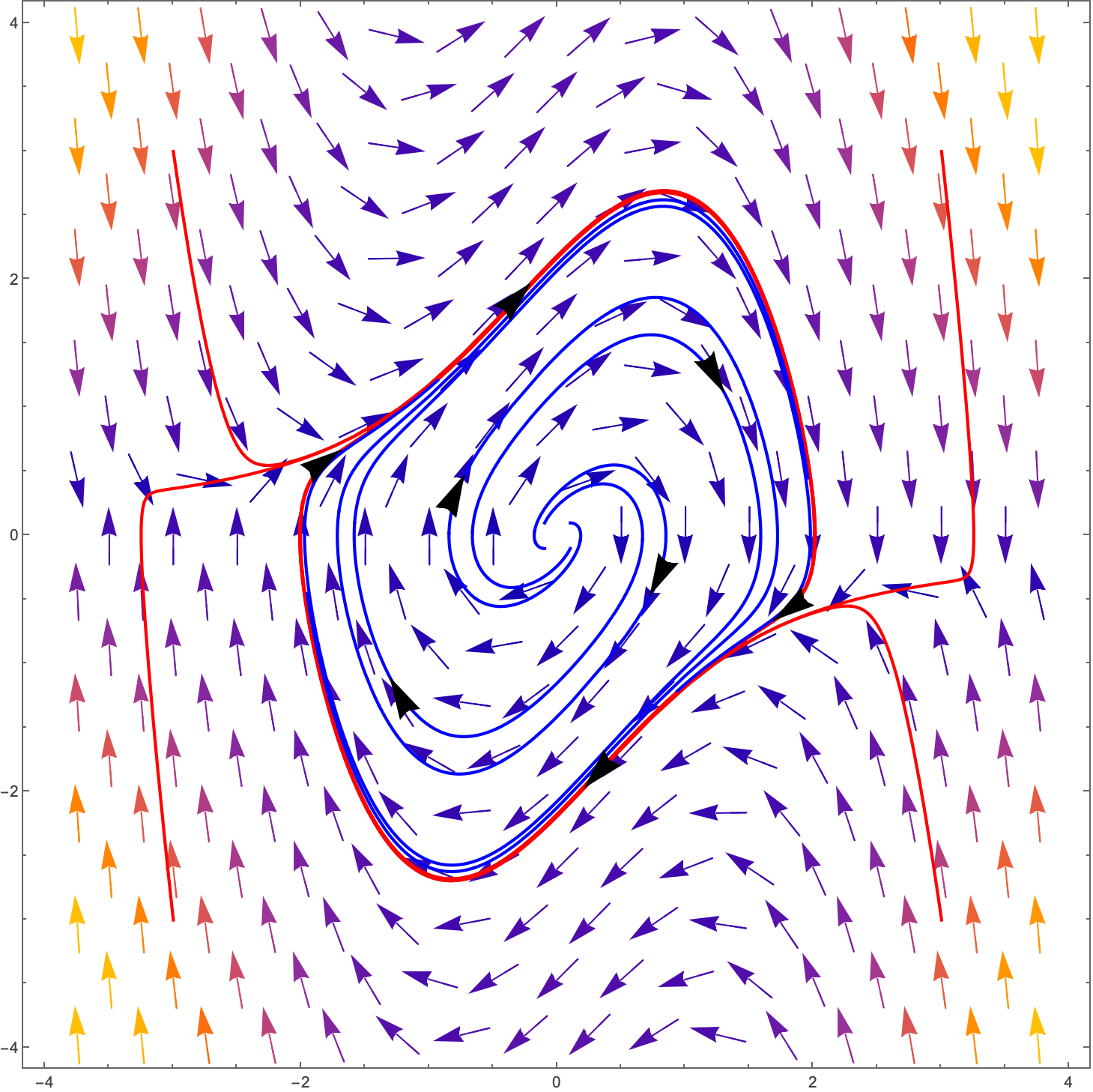
where we can see the limit cycle that everything is attracted to.

This particular case is for $\mu{}=1. $Can we say anything about the particular case where μ is very large? The term with μ is the only non-linear term in town, so turning up μ makes this really non-linear.

We can actually write the VDP equation in a slightly strange way as:

$$ \frac{d}{\text{ dt }}\left(\dot{x}+\mu{} \left(\frac{x^{3}}{3}-x\right)\right) =-x $$

Make sure that you can show this.

So by letting

$$ \dot{x}+\mu{} \left(\frac{x^{3}}{3}-x\right)=w $$

we have the two equations:

$$ \dot{x}=w-\mu{} \left(\frac{x^{3}}{3}-x\right) \left(\text{ just by } \text{ rearranging the } \text{ above equation }\right) $$

and

$$ \dot{w}=-x \left(\text{ just from } \text{ the definition } \text{ of } w \text{ above }\right). $$

Letting $w=\mu{} y$, we have:

$$ \dot{x}=\mu{} \left(y- \left(\frac{x^{3}}{3}-x\right)\right) $$$$ \dot{y}=\frac{-x}{\mu{}} $$

Note that you wouldn’t be expected to come up with this yourself, but you should be able to follow it.

How does this help anyone? Well, when μ is very large, this tells us that unless we are on the curve of

$$ y- \left(\frac{x^{3}}{3}-x\right)=0 $$

the thing that will be changing most is $x$, and $y$ won’t be changing quickly at all - so unless we are on the above curve, we will mostly move in horizontally, and fast, in the phase plane until we hit this curve…when we get really close to the curve, our $x$ speed will be slow too and we will start to move in both the $x \text{ and } y$ directions. Let’s just look at this for a moment. Plotting the curve we have:

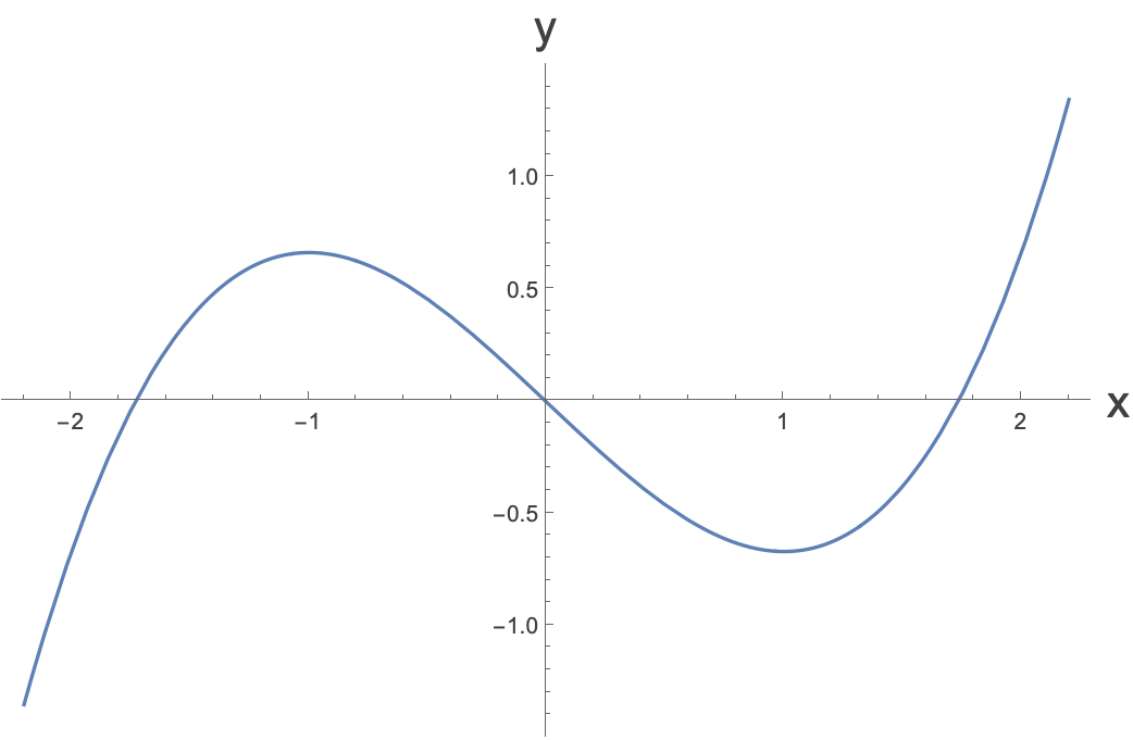
If we start off at the point, say $\left(0,0.5\right), $we have:

$$ \dot{x}=\mu{} \left(0.5- \left(\frac{0^{3}}{3}-0\right)\right) =0.5 \mu{} $$

which, for μ large means that we are moving fast in the positive $x$ direction. Remember that we will move very slowly in the $y$ direction.

In fact, we will keep moving quickly in the positive x-direction until we hit the curve, at which point we will stop moving any more in this direction. Then the motion will be slowly in the y-direction, and indeed it will be in the negative y-direction…that will take us just under the curve, which means that $\dot{x}$ will be negative, and we are starting, slowly, to move back in the negative x-direction. We will keep moving slowly in the negative x and y directions, hugging the curve.

But we can’t keep doing that forever. Once we get to the local minimum of the curve, the equation for the dynamics of y tells us that we will keep going more negative in y, but then we will have moved off the curve…and now $\dot{x}$ will be large and negative…so we will shoot back to hit the other side of the curve.

This is really a cartoon version of what will happen, but it’s close to the truth:

And so we will find ourselves in a stable limit cycle zipping left and right quickly, and then going slowly along the curve until we shoot off again to the other side.

Why is this a cartoon? Well, for one thing when we are going across, there will be some movement in the y-direction. It’s just that for large μ we can neglect it. The other major cartoonish thing that we ’ve done is to say that we move across to the right, then stop moving in the x-direction and just move a little in the y-direction until we are under the curve. In fact what happens here is that as we cross the curve (it’s a null-cline), we have to do so in the y-direction, but other than that when we are close to the curve we are moving at similar rates in the x and y-directions.

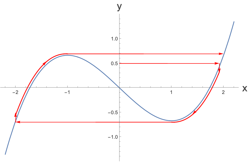
Let’s actually superimpose on top of this some trajectories for different values of μ, starting at the point (0,0.5) to see how close to the truth we were.

You can see that when $\mu{}=2$, the red cartoon drawing is not a good approximation of the true trajectory, in green. This isn’t surprising, because this isn’t a large value of μ. However, even for μ=5, we can see that it’s getting to be a pretty good approximation. Note that in the bits where we are whizzing across from left to right, there ’s a bit of vertical motion. But for μ=10, it looks like we are really very close indeed.

If we plot the trajectories of x and y, we see the following (x is in red and y is in blue):

Again, for large μ, we have periods of slow change in x, followed by sudden fast change in x. y on the other hand is always changing fairly slowly. If we go to even higher values of μ we see:

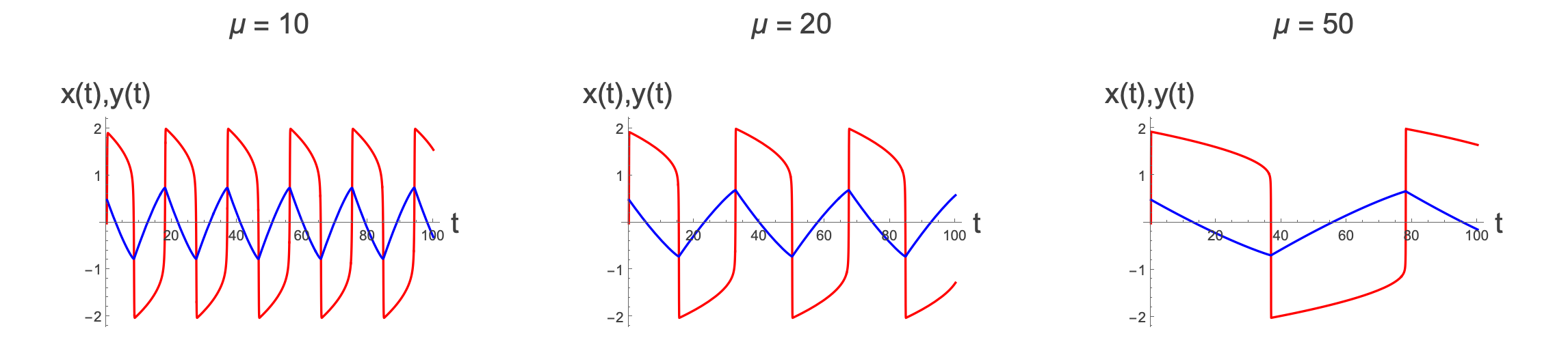
We see something particularly interesting here. It looks like when μ is large enough, we are just scaling the plot. For μ=10, we get five and a bit full oscillations in, whereas for μ=50, we just get one and a bit. There is a scaling behaviour here determined by μ. The timescale of the slow part of the trajectory is related to μ and the timescale of the fast part of the trajectory is related to $\frac{1}{\mu{}}$. We can see this because we know that the speed in the slow part of the trajectory is related to $\frac{1}{\mu{}}$ etc.

We denote this that the slow part of the cycle takes time $\Delta{}t\sim{}\mathcal{O}\left(\mu{}\right) \text{ and the } \text{ fast part } \text{ takes } \Delta{}t\sim{}\mathcal{O}\left(1/\mu{}\right) .$

Reminding ourselves of the animation in the previous section we see this behaviour and precisely where it is occurring, for $\mu{}=5$

Can we actually calculate the period in the limit of large μ for the Van der Pol system?

We know that there is a fast phase, and there is a slow phase…the fast phase is when we are not on the curve $y=\frac{x^{3}}{3}-x$ and the slow phase is when we are very close to it. If we want to calculate the period, then the slow phase is the most important part. So, we need to figure out how long we are on the curve for. To calculate how long something takes, you need to divide the distance by the velocity, but of course the velocity changes, so we do this as an integral.

$$ \text{ time to } \text{ go down } \text{ red arrow } = {\int{}}_{x_{a}}^{x_{b}}\frac{1}{\dot{x}}\mathrm{d}x $$

We have that along the curve:

$$ \dot{y}=\dot{x} \frac{d y}{d x}=\dot{x} \frac{d}{d x}\left(\frac{x^{3}}{3}-x\right)=\dot{x }\left(x^{2}-1\right) $$

so:

$$ \frac{1}{\dot{x }}=\frac{\left(x^{2}-1\right)}{\dot{y}} $$

But we know from the equation of motion that:

$$ \dot{y}=\frac{-x}{\mu{}} $$

So:

$$ \frac{1}{\dot{x }}=-\mu{}\frac{\left(x^{2}-1\right)}{x}=\mu{}\left(\frac{1}{x}-x\right) $$

Now we just need to figure out what are $x_{a} $and $x_{b}$, but these are found easily from the curve and are given by 2 and 1 respectively, so our integral is:

$$ \text{ time to } \text{ go down } \text{ red arrow } = {\int{}}_{2}^{1}\mu{} \left(\frac{1}{x}-x\right)\mathrm{d}x =-\mu{}{\int{}}_{1}^{2} \left(\frac{1}{x}-x\right)\mathrm{d}x=-\mu{}\left( \text{ ln }\left(2\right)-\frac{3}{2}\right)=\mu{}\left(\frac{3}{2}-\text{ ln }\left(2\right)\right) $$

The period in the large μ limit is thus twice this, plus corrections for the fast part, which turns out to be $O\left(\frac{1}{{\mu{}}^{\frac{1}{3}}}\right)$, so we have:

$$ T = \mu{}\left(3-\text{ ln }\left(4\right)\right)+O\left(\frac{1}{{\mu{}}^{1/3}}\right) $$

What a beautiful thing!

The next order term comes from the region where we are getting towards the curve, and slowing down and then getting onto the curve.