Section 2.2: Ruling out closed orbits

Section 2.2: Ruling out closed orbits

Strap in, things are about to get mathsy! We’re going to get into some slightly more complicated mathematical notation than we have before. You should have seen all of it, but I’ll try and explain it as well as possible as we go along.

Remember back last year we were able to show that dynamical systems in one dimension (ie. first order, no time-dependence) could not have oscillations?

We are going to prove something similar in two dimensions for a particular class of systems.

We already know that there do exist systems in two dimensions which do oscillate - ie. they have closed orbits. It turns out that a dynamical system in two dimensions which can be written in a particular way can never have closed orbits.

A system which can be written as:

$$ \dot{x}=-{\partial{}}_{x}V\left(x,y\right) $$$$ \dot{y}=-{\partial{}}_{y}V\left(x,y\right) $$

for some $V\left(x,y\right)$ cannot have closed orbits. We can actually write this in vector notation as:

$$ \dot{x}=-\nabla{}V\left(x,y\right) $$

where ∇=(${\partial{}}_{x}$,${\partial{}}_{y}$).

Such systems are called gradient systems as ∇ is the gradient operator, and when applied to a function gives a vector which is the gradient of the function in the basis directions.

To prove this, let’s assume that we have a system which is a gradient system, but there is a closed orbit. Moving along the closed orbit, the value of the potential will change, but if we start and end at the same point, then the total change in the potential, $\Delta{}V$, must be zero, as the potential is just a single-valued function of $x \text{ and } y$.

If you walk a little way along the path (say from time 0 to time t) of the closed orbit, you can calculate how much V has changed by doing a path integral:

$$ \Delta{}V={\int{}}_{0}^{t}\frac{d V}{d t}\mathrm{d}t $$

If you walk around the whole path, which has, say period $T, \text{ then } $this will give

$$ \Delta{}V={\int{}}_{0}^{T}\frac{d V}{d t}\mathrm{d}t $$

which we know from the above argument has to be zero on the left hand side. But let’s look at the right hand side. V itself is a function of $x \text{ and } y$ which along a path are themselves functions of t, so we can write:

$$ \frac{d V}{d t}=\frac{\partial{} V}{\partial{} x}\frac{d x}{d t}+\frac{\partial{} V}{\partial{} y}\frac{d y}{d t}={\partial{}}_{x}V \dot{x}+{\partial{}}_{y}V \dot{y} = \nabla{}V. \dot{x} $$

so the above integral is

$$ \Delta{}V={\int{}}_{0}^{T}\left(\nabla{}V. \dot{x}\right)\mathrm{d}t $$

but for a gradient system we have that

$$ \dot{x}=-\nabla{}V\left(x,y\right) $$

so that:

$$ \Delta{}V=-{\int{}}_{0}^{T}\left(\dot{x}. \dot{x}\right)\mathrm{d}t=-{\int{}}_{0}^{T}\dot{|x}|^{2}\mathrm{d}t $$

where remember $\dot{x} \text{ is the }$ vector rate of change of $x \text{ and } y$ along the path. So long as we aren’t at a fixed point, then this can’t be zero, and therefore because we have a square on the right hand side inside the integral, the right hand side can ’t be zero. But we know that the left hand side is zero, so we have a contradiction. So it is impossible to have a path (which isn ’t just a trivial fixed point) for which $\Delta{}V=0$ which rules out any closed orbits in a gradient system.

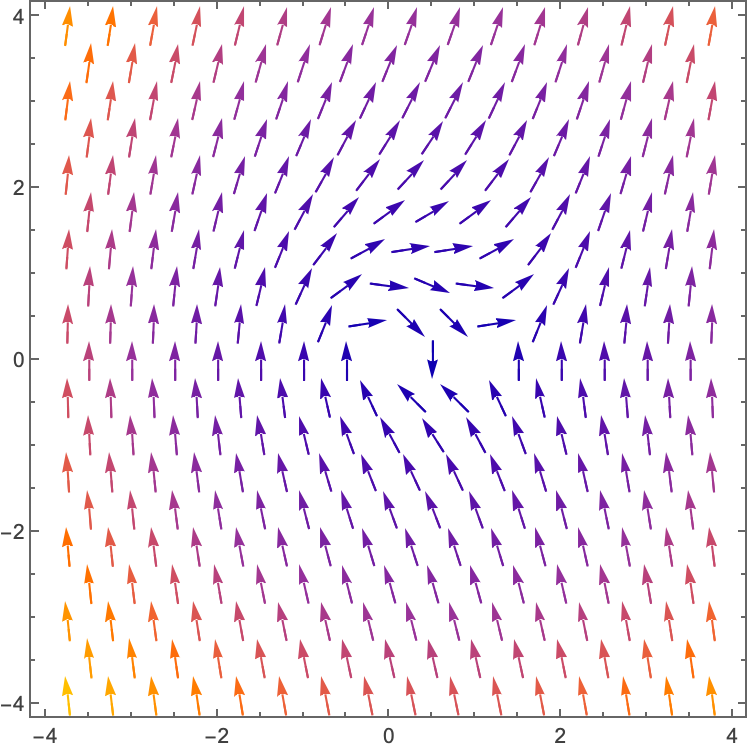
Now we can look at an example and prove that because it is a gradient system, it can’t have closed orbits. For instance:

$$ \dot{x}=\text{ sin } y $$$$ \dot{y}=x \text{ cos } y $$

This can clearly be written like

$$ \dot{x}=-\nabla{}V\left(x,y\right), \text{ for } V=-x \text{ sin } y $$

Plotting the vector field for this example we see

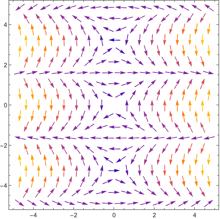
Which in this part of the phase plane doesn’t have any closed orbits, and you should be able to convince yourselves that in fact in no part of the phase plane could it have any (look at the periodicity in the y-direction in the phase plane, and what happens as you scale $x.$

In general if we have a system of the form

$$ \dot{x}=f\left(x,y\right) $$$$ \dot{y}=g\left(x,y\right) $$

Then if this is a gradient system we can ‘partially ’ integrate:

$$ -{\partial{}}_{x}V\left(x,y\right)=f\left(x,y\right) $$$$ -{\partial{}}_{y}V\left(x,y\right)=g\left(x,y\right) $$

And if these both give the same $V\left(x,y\right) \text{ then }$ we have a gradient system. Try this with

$$ \dot{x}=y^{2}+y \text{ cos } x $$$$ \dot{y}=2x y+\text{ sin } x $$

Note that we have said that being a gradient system implies that there are no closed orbits, but we haven’t said anything about the implication the other way. There can indeed be non-gradient systems which also have no closed orbits, and this can often be proved in a similar way.

Take the example

$$ \dot{x}=y $$$$ \dot{y}=-x-y^{3} $$

This is clearly not a gradient system, but we can write an energy function (you shouldn’t be able to see this from the above equations immediately):

$$ E=\frac{1}{2}\left(x^{2}+{\dot{x}}^{2}\right)=\frac{1}{2}\left(x^{2}+y^{2}\right) $$

where

$$ \dot{E}=x \dot{x}+y \dot{y}=x y+y\left(-x-y^{3}\right)=-y^{4}=-{\dot{x}}^{4}\leq 0 $$

and it’s only zero for a fixed point.

What this means is that for any trajectory which isn’t a fixed point, the energy of our system is decreasing. In fact this is the dynamical system for a damped harmonic oscillator $\left(\ddot{x}+{\dot{x}}^{3}+x=0\right)$, so it makes sense that the energy of the system always decreases.

Considering a closed cycle (we will use closed cycle/orbit interchangeably) in this system $\Delta{}E$ around the cycle must be zero, for the same reason as with ΔV above. We can write the change as:

$$ \Delta{}E={\int{}}_{0}^{T}\dot{E}\mathrm{d}t=-{\int{}}_{0}^{T}{\dot{x}}^{4}\mathrm{d}t\leq 0 $$

So we have that $\Delta{}E=0$ and $\Delta{}E\leq 0$ which is a contradiction, so we can’t have closed cycles in this system.

Liapunov/Lyapunov functions

This is the first time in this course, or the previous one we have mentioned the name Lyapunov, but it will come up a number of times as we go on, in particular when we get on to chaos.

In the previous example we were able to show the absence of closed cycles by finding an energy function which always decreased along non-fixed-point trajectories. In fact we can generalise this that any system for which we can find a positive function, $V\left(x\right)$, of the phase space coordinates away from a fixed point at $x^{*}$:

$$ V\left(x\right) \begin{cases} >0, & \text{ for } x\neq x^{*} \\ =0, & \text{ for } x=x^{*} \end{cases} $$

and where the rate of change of $V\left(x\right)$ is negative along trajectories:

$$ \dot{V} \begin{cases} <0, & \text{ for } x\neq x^{*} \\ =0, & \text{ for } x=x^{*} \end{cases} $$

then we can say that there are no closed orbits and $x^{*}$ will be globally asymptotically stable. This means that wherever you start in this system, you will always end up at $x^{*}$. That is:

$$ x\left(t\right)\to x^{*} \text{ as } t\to \infty{} $$

The reason for this is that because you must always move along trajectories such that $V \text{ is decreasing }$, there’s no way of getting stuck at any point except $x^{*}$ as if you did, $\dot{V}$ would be zero, and we know that it can’t be except at the fixed point.

Finding this Lyapunov function, $V$, is generally very hard, if it’s possible at all and there is no systematic way of finding one.

As a true aside, there is something similar that shows up in high energy theoretical physics (in particular quantum field theory) called a c-theorem, but we are not going to go into that here…

Dulac’s criterion

We’re going to show one other way to prove that a system can ’t have any closed orbits.

To show this we will have to use Green’s theorem. I’m going to write it out in words, which is going to seem super complicated, but we will break it down after and see what it means:

This last part means that we take the vector at the boundary, and take the component of it in the direction normal to the boundary and then integrate that along the boundary - moving counterclockwise.

That is, given some continuously differentiable (it only has to be so within the region of interest) vector field, let’s call it $v$****(not the same as the potential, just some vector field) we can write the divergence of the vector field as

$$ \nabla{}. v $$

which in 2d is equal to

$$ {\partial{}}_{x}v_{x}+{\partial{}}_{y}v_{y} $$

ie. is a scalar quantity. The integral of this over some region in 2d is:

$$ \int{}{\int{}}_{R} \left({\partial{}}_{x}v_{x}+{\partial{}}_{y}v_{y}\right)d A $$

where $ d A \text{ is just } \text{ adding up } \text{ the bits } \text{ of the } \text{ area over } R, \text{ is } $the region over which we are integrating. This is just the area under the surface of the scalar function ${\partial{}}_{x}v_{x}+{\partial{}}_{y}v_{y}$.

Green’s theorem says that this is equal to the dot product of $v \text{ with the } \text{ normal }$ to the boundary

$$ \int{}{\int{}}_{R} \left({\partial{}}_{x}v_{x}+{\partial{}}_{y}v_{y}\right)d A={\oint{}}_{\partial{} R}v.n d l \text{ which is } \text{ equivalent to }: $$$$ \int{}{\int{}}_{R} \nabla{}. v d A={\oint{}}_{\partial{} R}v.n d l $$

where $l$ parameterises the path along the boundary and C labels the boundary of $R.$

Let’s just look at a quick example of this. Taking the vector field

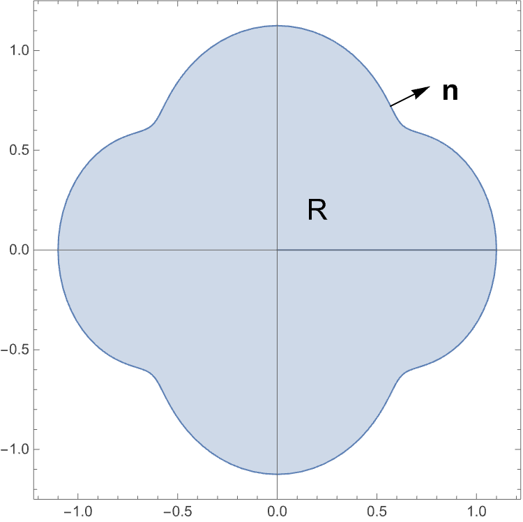
$$ v=\left(\begin{matrix} y \text{ sin } y \\ \text{ cos } y+x/2 \end{matrix}\right) $$

and taking some region given in blue below, we plot the vector field, some region R, and the unit normal to the boundary of the region given by the black arrows:

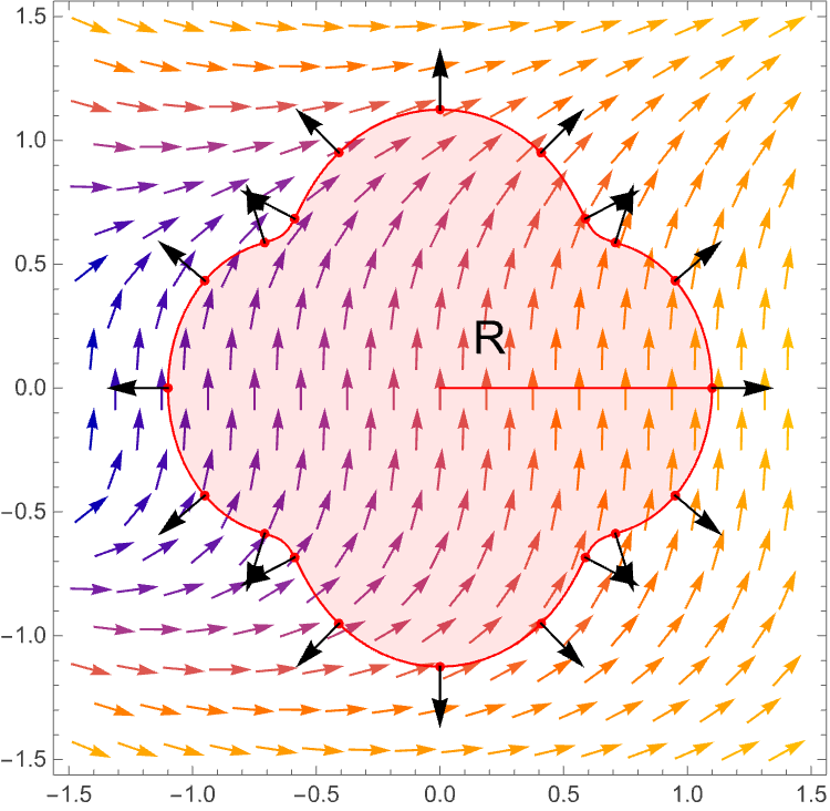
Note that the vector field, and the region are arbitrary other than the fact that the vector field is continuously differentiable in $R$ and the region $R$ has a well defined normal to it at all points on its boundary.

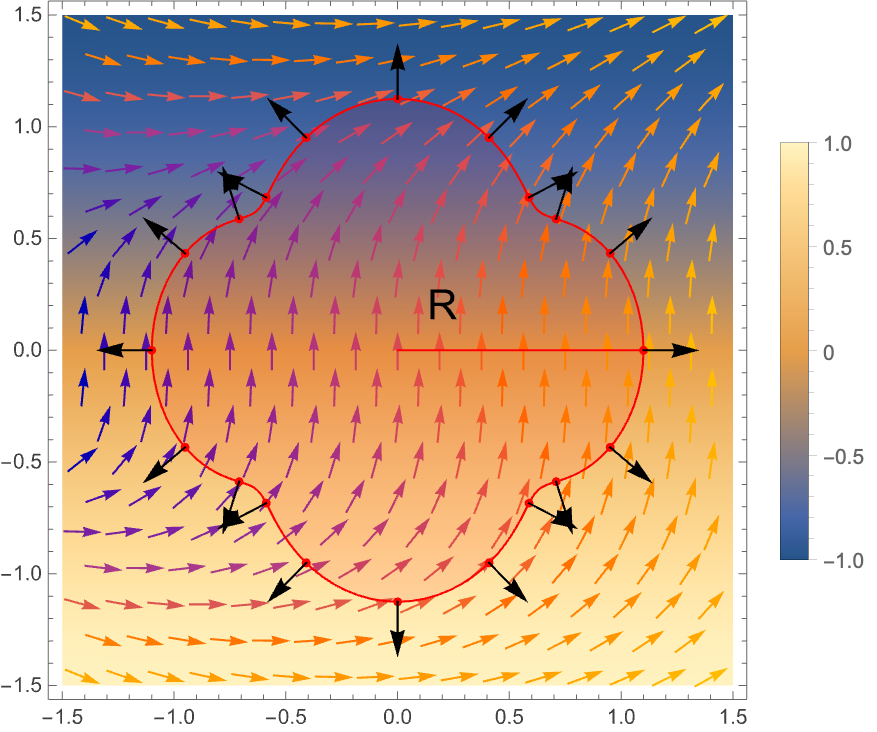
The scalar field

$$ \nabla{}. v={\partial{}}_{x}v_{x}+{\partial{}}_{y}v_{y}=-\text{ sin } y $$

Which we now overlay on top of the above plot as a heat map (ie the colours indicating values between -1 and 1).

Green’s theorem says that if we take the dot product of the field lines along the boundary of R with the unit normal vectors along this boundary and integrate them, then that will be the same as the surface integral of the $\nabla{}.v$.

OK, so that’s Green’s theorem, which is incredibly powerful, but we aren’t going to prove it here. It’s probably a lot to take in so don’t stress about it too much for the moment. We are however going to use it.

Now on to Dulac’s criterion

Let’s say that we have some vector field describing a dynamical system

$$ \dot{x}=f\left(x,y\right) $$

and the function $f $is continuously differentiable on a connected region $R$ (connected here is a term from topology, but just think of it as some region which isn’t split into disconnected islands).

If there exists some continuously differentiable, function $g\left(x\right)$ in the reals such that

$$ \nabla{}. \left(g\left(x\right)f\left(x\right)\right) $$

is always either always positive or always negative in $R$ then there can be no closed orbits which are entirely within $R$.

Note for a moment in the above expression which things are vectors and which are scalars. We can write it out purely in terms of scalars as:

$$ \left({\partial{}}_{x},{\partial{}}_{y}\right). \left(g\left(x,y\right)\left(f_{x}\left(x,y\right),f_{y}\left(x,y\right)\right)\right)={\partial{}}_{x}\left(g f_{x}\right)+{\partial{}}_{y}\left(g f_{y}\right) $$

where we’ve written $f=\left(f_{x},f_{y}\right).$

Again we are going to prove this by contradiction and we are going to use Green’s theorem where will use $v=g\left(x\right)f\left(x\right)= g\left(x\right) \dot{x}$ as our vector field.

Let’s assume that there is some closed orbit, $C, $that lies entirely within $R$. Let $A$ be the region inside the closed orbit. Then we can apply Green ’s theorem to the region within the closed orbit:

$$ \int{}{\int{}}_{A} \nabla{}. \left(g\left(x\right) \dot{x}\right) d A={\oint{}}_{C}\left(g\left(x\right) \dot{x}\right).n d l $$

We stated that $\nabla{}. \left(g\left(x\right) \dot{x}\right)$ always took on one sign on $A$ (ie. always positive or always negative), and so the right hand side of this expression is certainly non-zero.

The right hand side can be written as:

$$ {\oint{}}_{C}g\left(x\right)\left( \dot{x}.n \right)d l $$

But the region here is the supposed closed orbit, so $\dot{x}$ is always going to be tangential to the orbit. On the other hand $n$ is always going to be normal to the orbit, so we must have that $\dot{x}.n=0$. So the right hand side of the equation must be zero. So again we have a contradiction.

Just to give a bit more of a picture here, we are saying that we have some vector field $g\left(x\right) \dot{x}$ with a particular property related to the sign of its gradient in some region R. Then within that region we are suggesting that there might be a closed orbit. We then apply Green’s theorem not to R, but to the closed orbit, and show that there is a contradiction, and so there can be no closed orbit within R.

The trick to Dulac’s criterian is that finding $g\left(x\right) \text{ may be } \text{ very hard }.$ I’m going to show you an example, but you wouldn ’t be expected to find this function $g.$

Given a vector field:

$$ \dot{x}=\left(\begin{matrix} y \\ -x-y+x^{2}+y^{2} \end{matrix}\right) $$

If you take

$$ g\left(x\right)=e^{-2x} $$

Then the vector field $\dot{x}$ g(x) has gradient:

$$ \nabla{}. \left(g\left(x\right) \dot{x}\right)={\partial{}}_{x}\left(e^{-2 x}y\right)+{\partial{}}_{y}\left(e^{-2x}\left(-x-y+x^{2}+y^{2}\right)\right)=-2 e^{-2x}y+e^{-2 x}\left(-1+2y\right)=-e^{-2 x} $$

Which is negative for any value of $\left(x,y\right), $so in this case we can say that there are no closed orbits at all.

Note, that this doesn’t say that there can ’t be fixed points, and indeed there are two of them at $\left(x,y\right)=\left(1,0\right),\text{ and } \left(0,0\right)$.

Note that naively it looks like there might be closed orbits, but zooming into the region around the origin gives:

ie. an ingoing spiral. Check that this is the case by linearising the system.

What is the intuition behind Dulac’s criterion?

First we need to talk about the divergence operator. What is $\nabla{}.$ telling us when applied to our vector field? $\nabla{}. \dot{x}$. The divergence operator tells us about how much the space is getting stretched at a point - how much it is pushed and pulled, in contrast to the curl, which tells us how much it is twisting. For a closed orbit, we can think that there must be a balance between pushing and pulling. In some places it may be pushed out from the centre, in others it may be pulled in, but overall it should cancel out.

If we can find a quantity$ g\left(x\right)\dot{x}$ whose divergence is always positive (or always negative) then it has to be that as you go around a closed loop, the total amount of pulling and pushing cannot cancel out for this particular quantity and therefore it is not possible to have this careful balance which can lead to a closed loop.

OK, so next we are going to move on to showing that there are closed orbits….