Section 2.1: Limit Cycles

Section 2.1: Limit Cycles

We’re going to start with an example here.

Taking the vector field in polar coordinates:

$$ \dot{r}=r \left(1-r^{2}\right) $$$$ \dot{\theta{}}=1 $$

and converting these to Cartesian coordinates:

$$ \dot{x}=x-x^{3}-y-x y^{2} $$$$ \dot{y}=y-y^{3}+x-y x^{2} $$

we can plot the vector field in the Cartesian plane along with some trajectories.

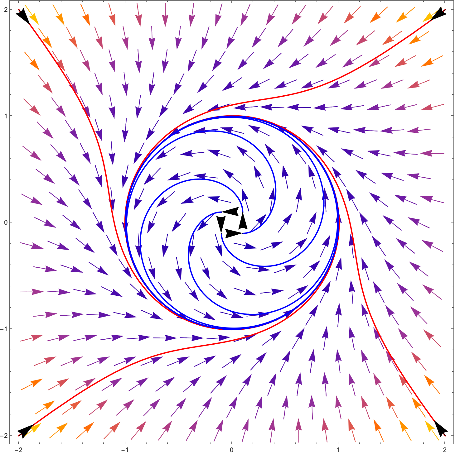
We see that this system has a center, at $r=1. If \text{ we start }$ outside the center, then we spiral towards it. If we start inside the center then we also spiral towards it. The center seems to be attracting trajectories both outside it and inside it.

This circular trajectory is called a limit cycle. The limiting behaviour of those trajectories spiraling in are the limit cycle. This is a stable limit cycle, but you can have unstable limit cycles (imagine just changing $t\to -t$ in the above), where the trajectories are repelled from it, and semi-stable limit cycles where only the inside or the outside flow towards the cycle, and the other flows away.

An example of a semi-stable limit cycle is given by the vector field

$$ \dot{r}={\left(1-r\right)}^{2} $$$$ \dot{\theta{}}=1 $$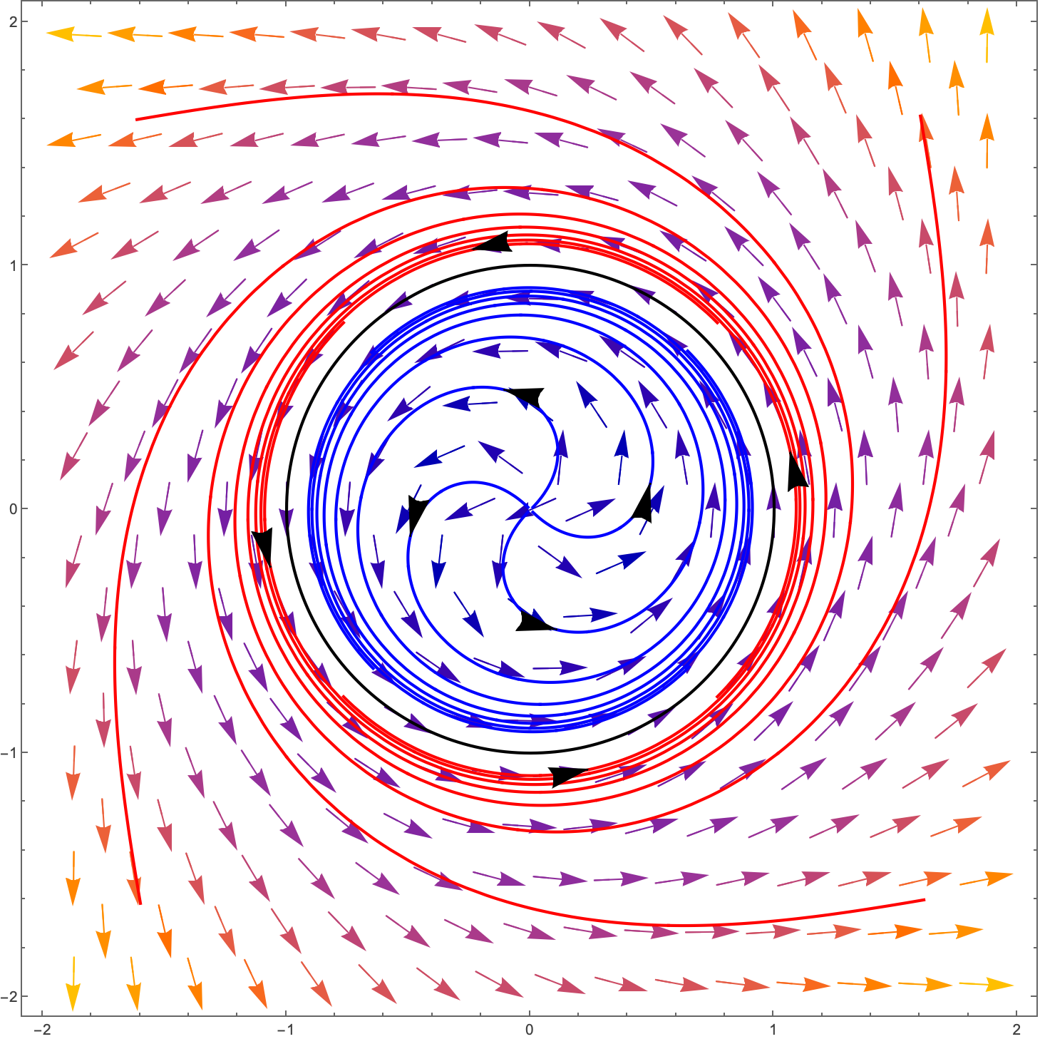

Any trajectory which starts within the limit-cycle of radius 1 is attracted to it, and any trajectory which starts outside the cycle is repelled from it.

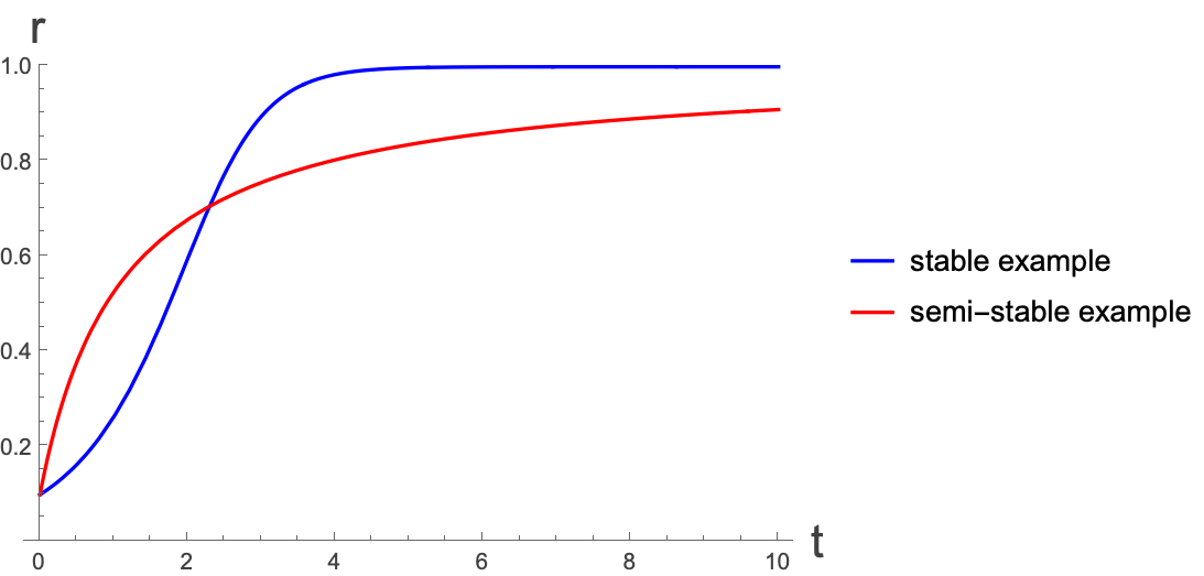
As an aside, take a look at the vector fields above (both cases) in polar coordinates and see if you can understand the phase diagram intuitively. The fact that the system is decoupled should allow you to understand what is going on quite clearly. In fact, in polar coordinates you can solve these systems exactly and see that the example of the stable fixed point goes towards the cycle much more quickly (in the long term) than in the semi-stable example. This isn’t a general principle of stable and semi-stable fixed points, but might be something that you wonder about from the trajectories above.

**Exercise:**For the above vector fields, try and plot $x\left(t\right) $for a number of different starting conditions.

So how come we never saw these types of behaviour when we looked at linear systems last year? Remember we did have stable and unstable spirals, but nothing where we had solutions which spiralled towards a circle. There ’s a very clear reason for this not being possible in a linear system.

$$ \left(\begin{matrix} \dot{x} \\ \dot{y} \end{matrix}\right)=A\left(\begin{matrix} x \\ y \end{matrix}\right) $$

where remember $A$ is 2x2 matrix. Let’s say now that we have some solution given by

$$ \left(\begin{matrix} x^{\text{ circ }}\left(t\right) \\ y^{\text{ circ }}\left(t\right) \end{matrix}\right) $$

where this is just some circular trajectory, let’s say with radius $r$. Because of linearity, anything of the form

$$ a \left(\begin{matrix} x^{\text{ circ }}\left(t\right) \\ y^{\text{ circ }}\left(t\right) \end{matrix}\right), a\in{} R $$

will also be a solution. This is just a scaling of the original trajectory, and so corresponds to a circle of radius $a r$. This means that if you have a circle solution, then ALL solutions will be circles. Remember we can’t have an intersection of trajectories, so either everything is a circle, or nothing is a circle.

This then shows that in a linear system you couldn’t have a circle, and a spiral trajectory.

The Van Der Pol Oscillator

We’ve looked previously at driven and damped systems. They tend to be systems of the form

$$ \ddot{x}+\mu{} \dot{x}+x=0 $$

where when $\mu{}=0$ we just have simple harmonic motion. When $\mu{}>0$ we have damped harmonic motion and when we have $\mu{}<0$ we have driven harmonic motion.

Check that the matrix of the coupled first order system of the above equation is given by:

$$ A=\left(\begin{matrix} 0 & 1 \\ -1 & -\mu{} \end{matrix}\right) $$

For instance, when we have initial conditions $x\left(0\right)=1, x'\left(0\right)=-1/2$, the solutions for $\mu{}=\pm{}1$ are:

$$ x_{\mu{}=1}= {\mathrm{e}}^{-t/2} \text{ cos }\left(\frac{\sqrt{3} t}{2}\right) $$$$ x_{\mu{}=-1}= {\mathrm{e}}^{t/2} \left(\text{ cos }\left(\frac{\sqrt{3} t}{2}\right)-\frac{2}{\sqrt{3}} \text{ sin }\left(\frac{\sqrt{3} t}{2}\right)\right) $$

Make sure that you can see why one is driven and one is damped.

So in this case depending on the parameter $\mu{}$ the system is either driven, or damped, but can’t be both.

How about if the driving/damping term were itself dependent on $x?$ Well, the Van der Pol oscillator (a model which has been used for electrical circuits, seismology and the firing of neurons in the Fitzhugh-Nagumo model) is given by:

$$ \ddot{x}+\mu{} \left(x^{2}-1\right) \dot{x}+x=0 $$

where we can see that for positive μ, depending on whether $x^{2}-1$ is greater than or less than 0 we are going to have damping or driving.

Writing this as a coupled system we have

$$ \dot{x}=y $$$$ \dot{y}=-x-\mu{}\left(x^{2}-1\right)y $$

Think about the effect that this non-linear term might have.

Below is plotted the phase plane with some trajectories for this system:

While there is no circular solution here, there is a stable limit cycle which both trajectories starting inside it and those starting outside it are attracted to.

There’s a full lecture by Steven Strogatz here on the Van der Pol oscillator which is very good, though you don ’t need to know all of the details for this course.