Section 1.6: Index Theory
Section 1.6: Index Theory
In this section we are going to develop some tools to allow us to say things about large scale, or global properties of a phase portrait. So far we have been able to zoom in on what is happening at, or close to a fixed point, but it would be useful to be able to talk about larger-scale properties of the dynamics of a system. This is going to seem a bit abstract at first, but stick with it and we will end up with some very powerful technology.
Imagine drawing some closed curve in a phase portrait. It can be any curve, so long as it’s closed and it doesn’t self-intersect.
Now walk along that curve and as you do so look at the vector field at each point. Each of the vectors makes some angle with the x-axis. Let ’s see what we mean by this with one particular point on a particular curve on a vector field.
Let’s take an example from section 1.1:
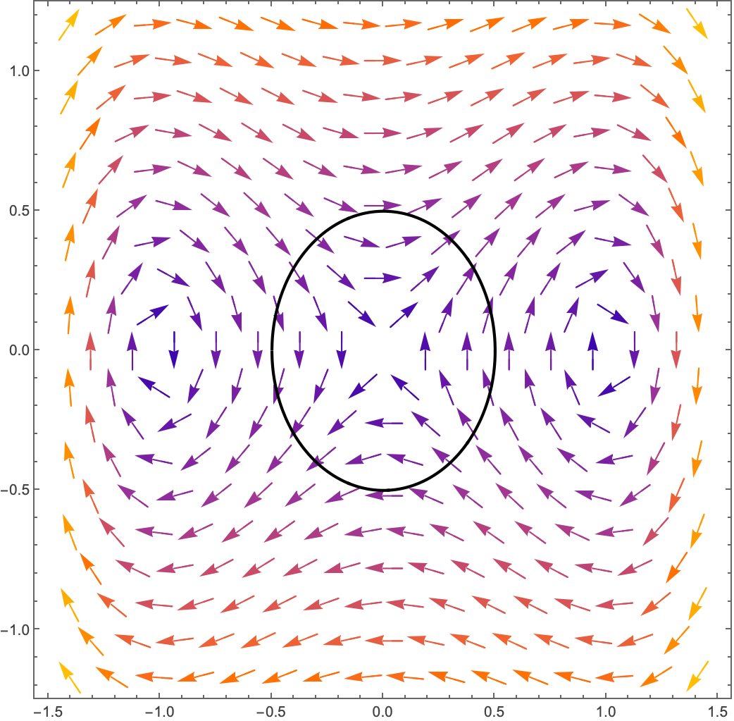
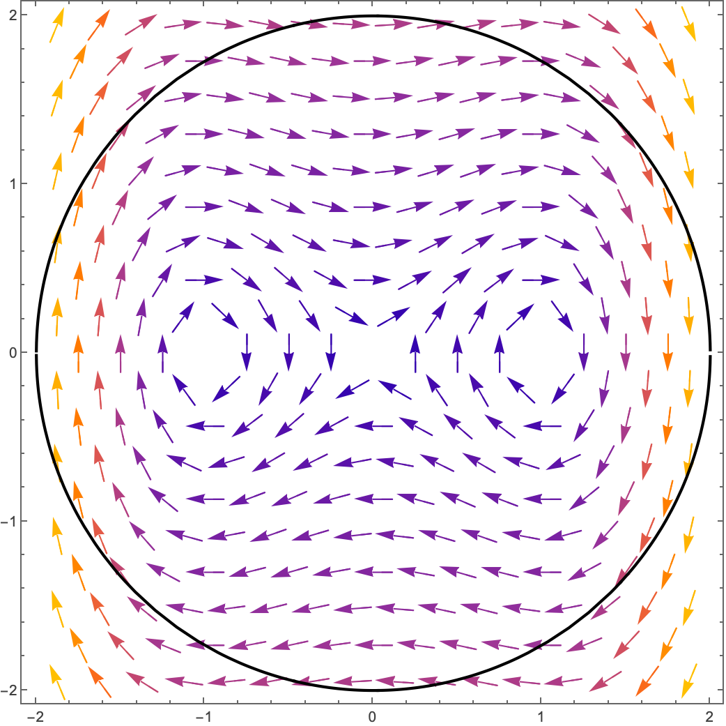
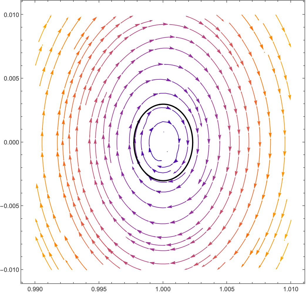
$$ {\dot{x}}_{1}=x_{2} $$$$ {\dot{x}}_{2}=x_{1}-{x_{1}}^{3} $$This is the vector field:
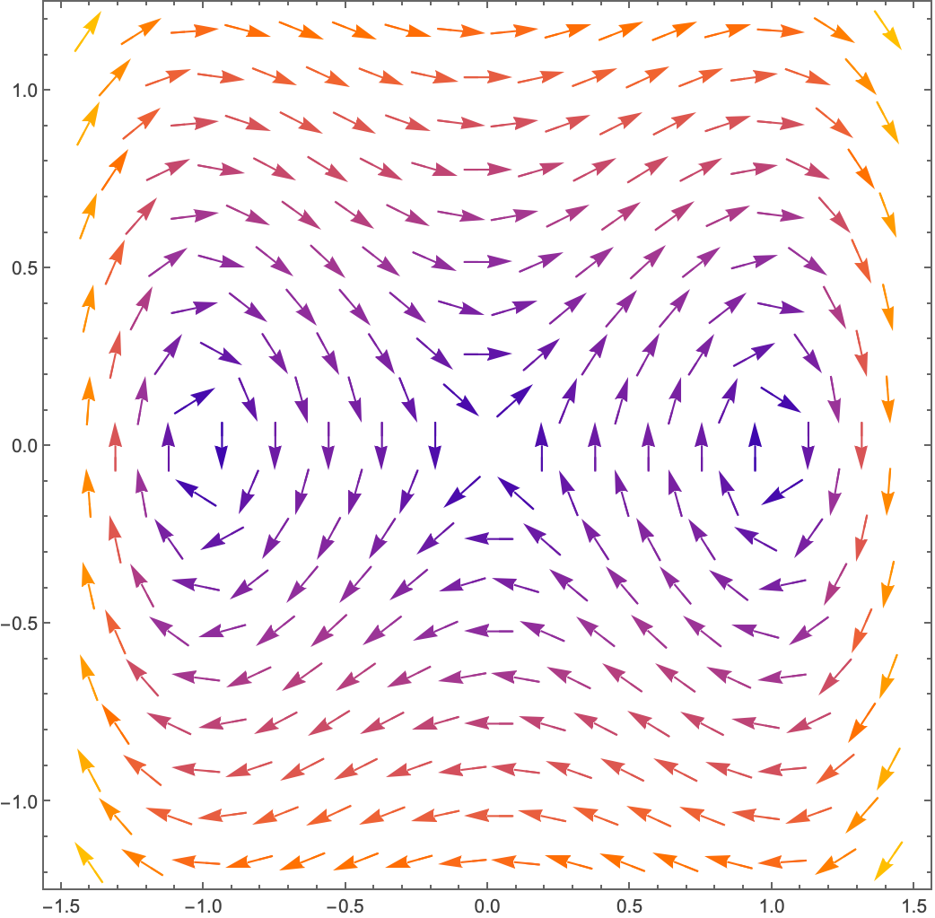
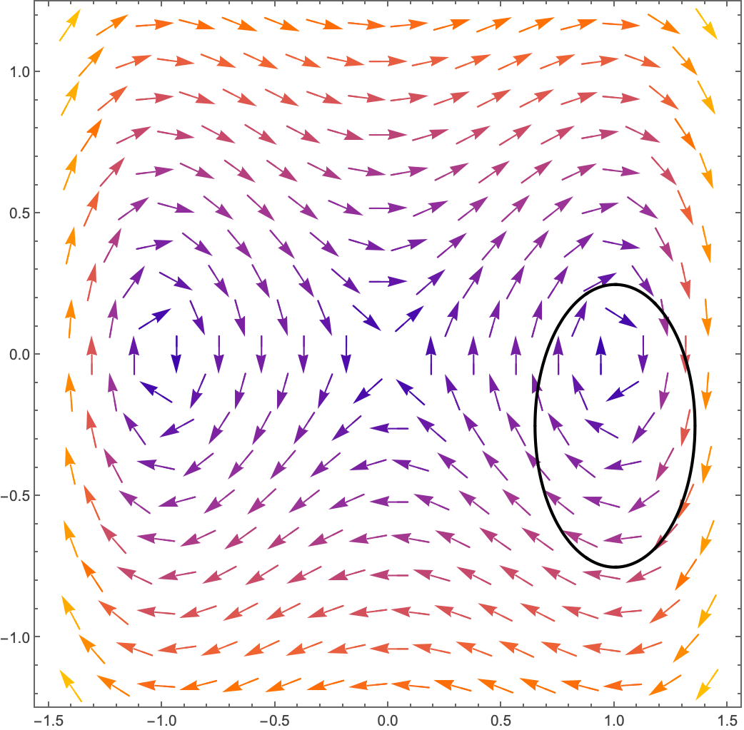
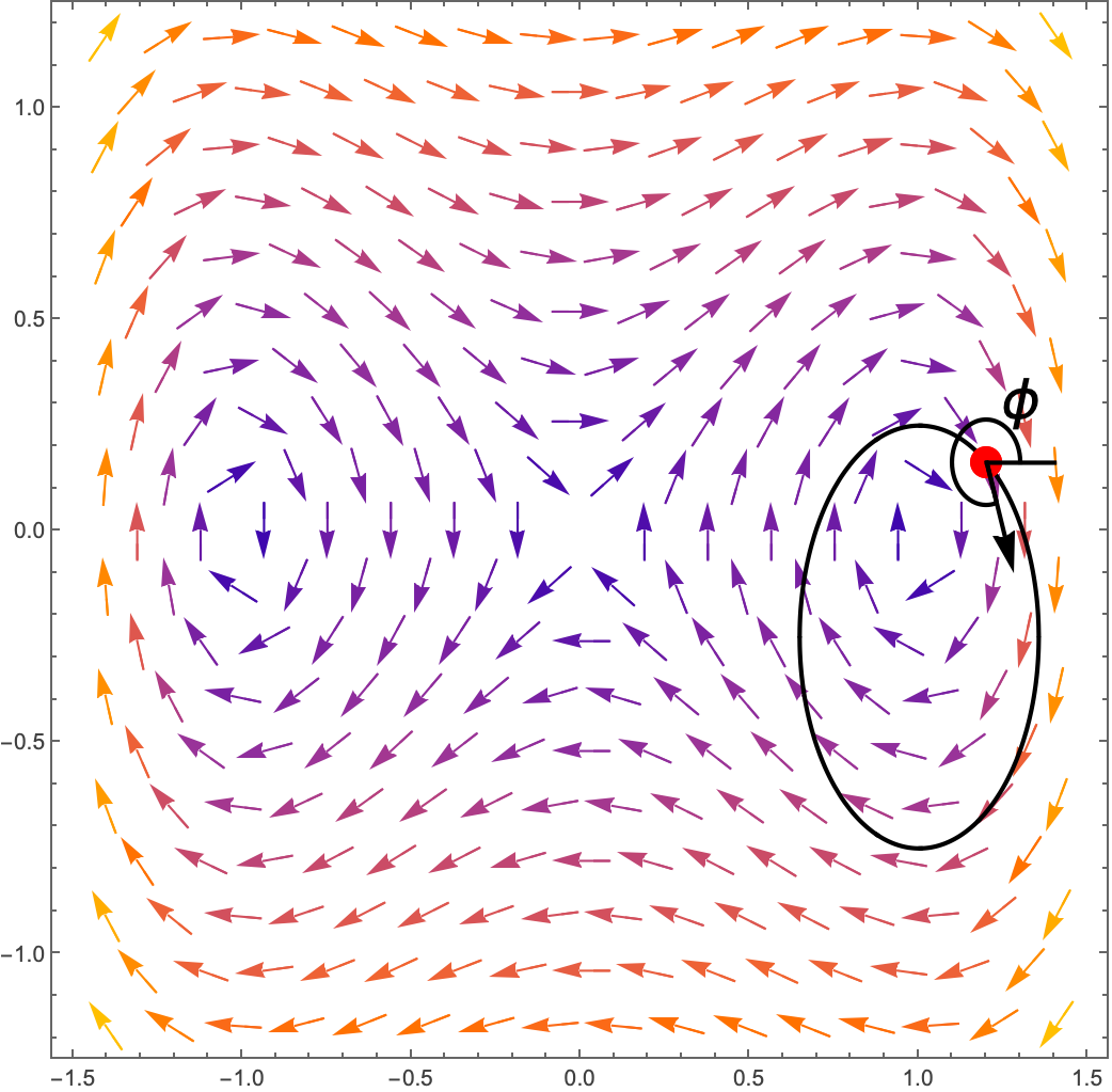
and let’s draw on some random closed curve, as shown:
and some point on the curve, say at $\left(1.2,\sqrt{{0.5}^{2}-2{\left(1.2-1\right)}^{2}}-0.25\right)=\left(1.2,0.1623\right)$:
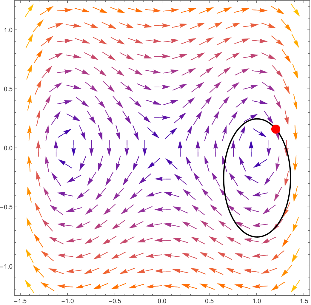
and the vector at that point which is:
$$ \left(\begin{matrix} x_{2} \\ x_{1}-{x_{1}}^{3} \end{matrix}\right)=\left(\begin{matrix} 0.1623 \\ -0.528 \end{matrix}\right) $$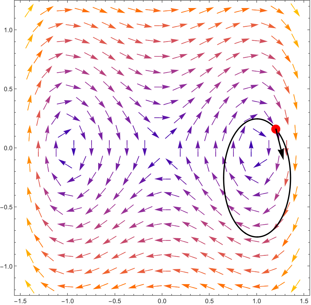
Now take that vector and calculate the angle with the positive x-axis (we ’ve written here -φ because we measure in the counterclockwise direction):
OK, so that seemed like quite a lot of work for one point, but actually we could have calculated that angle just from
$$ \phi{}={\text{ tan }}^{-1} \frac{{\dot{x}}_{2}\left(x_{1},x_{2}\right)}{ {\dot{x}}_{1}\left(x_{1},x_{2}\right)} $$or in the more usual language of $x \text{ and } y:$
$$ \phi{}={\text{ tan }}^{-1} \frac{\dot{y}\left(x,y\right)}{ \dot{x} \left(x,y\right)} $$where $x^{ } \text{ and } y $are the coordinates on the curve.
OK, so now imagine doing that as you walk counterclockwise around the whole curve…calculate this value φ as you do so.
Keep track of φ as you start at one point and return to the original point. Clearly φ will be the same where you started and where you stopped, so whatever φ did along the way, it will have moved by some integer number of times around a full rotation.
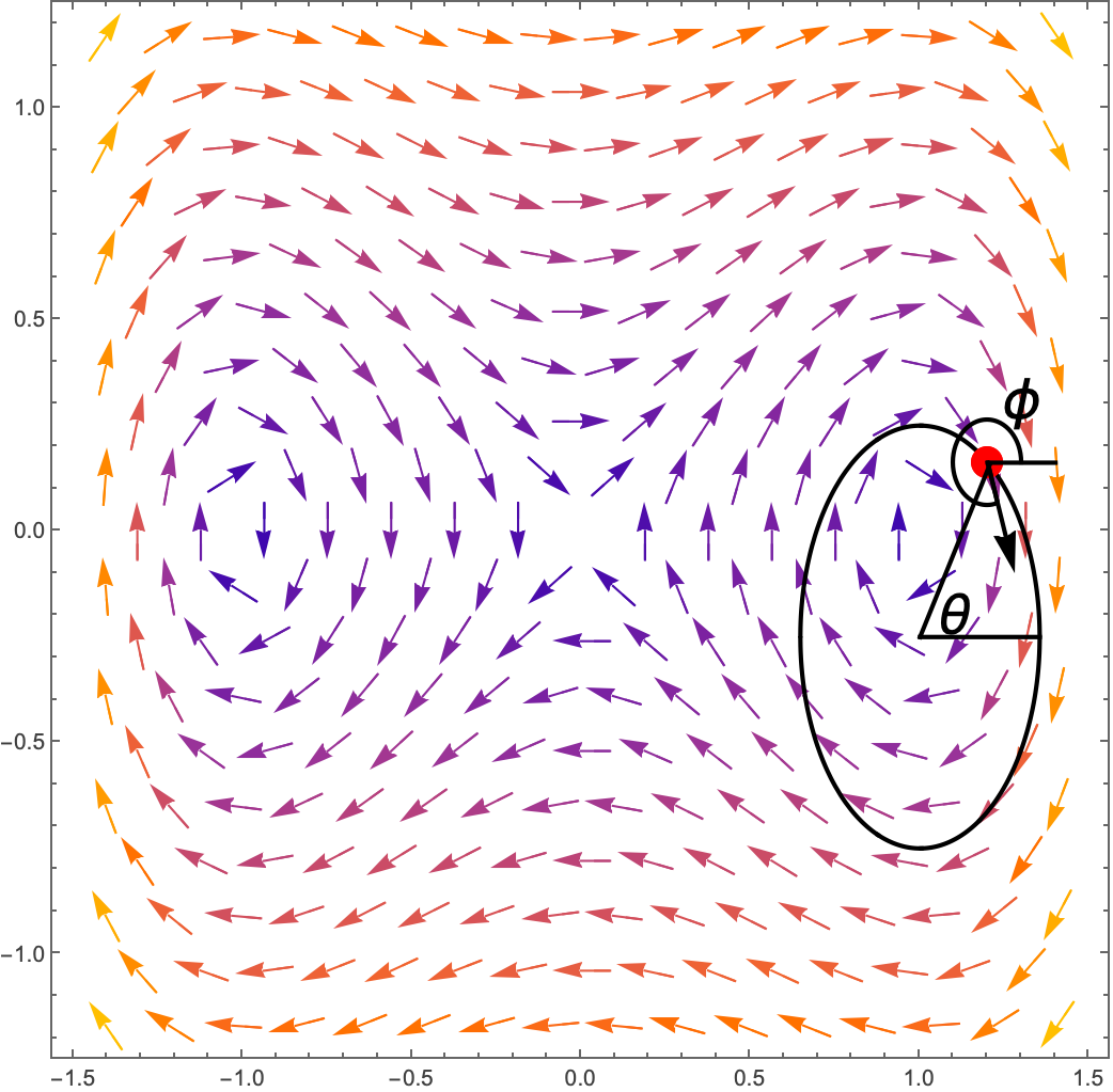
Let’s have a look at that as we traverse the loop above. On the right we have just plotted the vector on its own. We can see here that as we go around the closed loop, the vector does one full rotation.
Let’s think about plotting φ as we move around the curve. Let’s parameterise the curve by the angle θ as we move around it in a counterclockwise direction.
If we do this naively, it looks a bit strange:
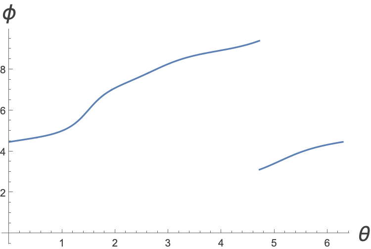
At θ=0, we’re pointing kind of down, which we can call φ[TildeTilde]$\frac{-\pi{}}{2}$ or we can call it φ[TildeTilde]$\frac{3\pi{}}{2}.$ Here we have chosen to call it the latter. As we increase θ, φ increases, but at around θ=-$\frac{3\pi{}}{2}$ we are pointing directly to the left, which we can call either $\phi{}=\pi{}$ or φ=-π, or φ=3π, etc. we have to remember that this is really continuous, so we could instead plot it like:
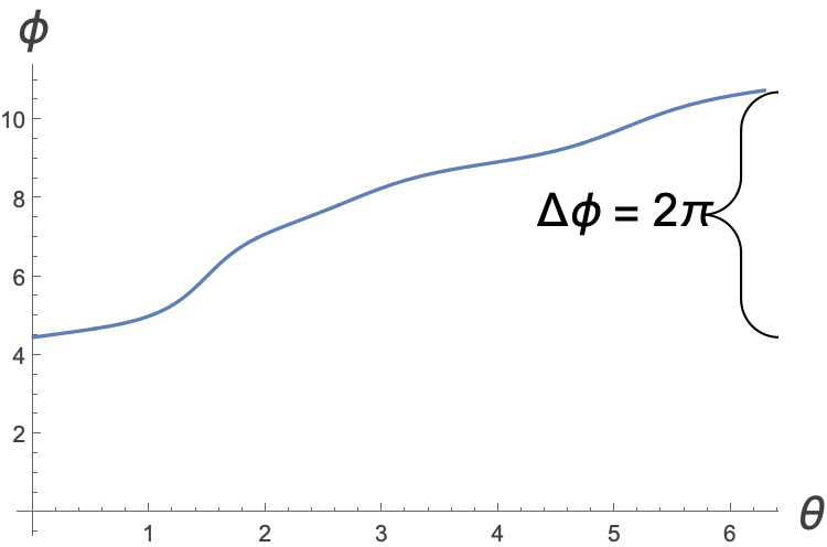
The important point is just the total change in φ as we move around the contour, and in this case it is 2π.
Was that necessarily the case? Well, how about we try the same thing but this time a loop in a different position.
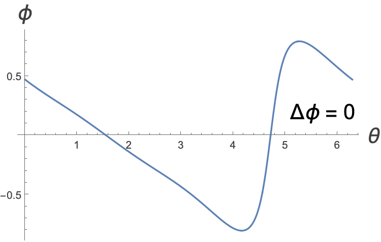
Well, in this case we see that as it goes around, the arrow doesn ’t do a full rotation at all - it certainly moves about, but it doesn’t ever point to the left.
Let’s do the same thing around this contour with φ as a function of θ.
Let’s do the same thing about the fixed point at the centre:
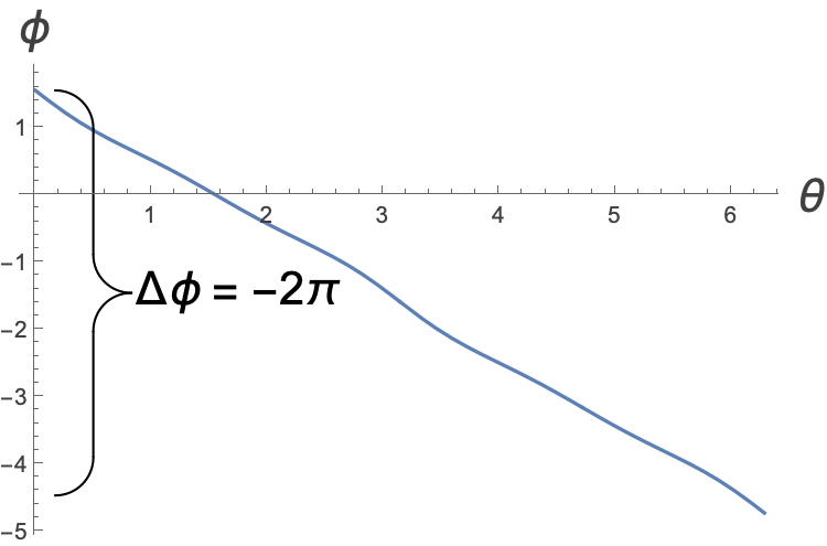
Intriguing! So in this case Δφ is -2π.
Now let’s go around all the fixed points:
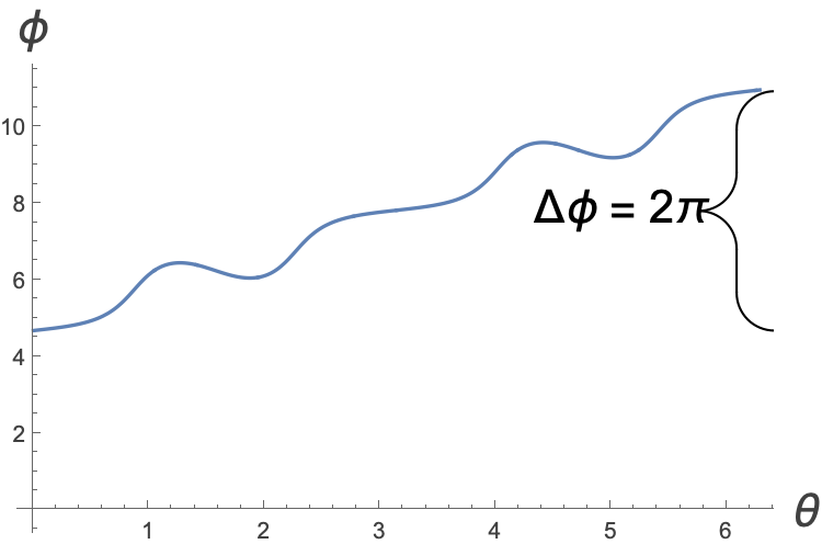
So we see here that we have gone around 2π again. But this is interesting because we are capturing three fixed points, two of which have Δφ=2π and one of which has Δφ=-2 π. And overall we have Δφ=2π…interesting.
OK, so I hope that you are convinced that whatever happens to this vector, it has to rotate around some integer number of times as we go around the closed loop.
Actually, we have to be a little bit careful, because if the loop ever touches a fixed point then the vector goes to zero and it doesn ’t make sense to talk about whether a zero vector has rotated or not, so we will constrain ourselves to loops which don ’t go through any fixed points.
So we’ve seen in the above example that with the first loop, the vector with angle φ rotates once, and with the second loop it doesn ’t rotate at all.
The difference between the two is that the first loop encircled a center fixed point, and the second one didn’t encircle any fixed point at all…hmmm…I smell a clue…
We denote the Index of the closed curve, C, with respect to a vector field as:
$$ I_{C}={\frac{1}{2\pi{}}\left[\phi{}\right]}_{C} $$Where ${\left[\phi{}\right]}_{C}$ is the total change in φ as you go around the closed curve.
The index counts the number of times the vector rotates as you follow the closed curve. In the first example about $I_{C}$ = 1 and in the second example $I_{C}=0.$
Exercise
Try and imagine what the index of the curve that just goes around the saddle point. How about something that goes around the saddle point and one of the centers? How about all the fixed points?
Given the following vector field and curve, calculate the index.
Do this by taking points at, for instance π/4 intervals around the circle, and write down which way the vector is pointing as you go around counterclockwise. Then write each of those direction vectors in a row and see how much it has rotated ‘net’, that is, if it goes π one way, then π the other, then net it has not rotated at all.
Properties of $I_{C}$
So the index of a curve seems to be telling us something about the fixed points inside the curve. This means that if we move the curve from $C$ to a new curve $C’$ in such a way that the fixed points within it remain the same, then the index shouldn’t change, ie. $I_{C}=I_{C’}$. Remember that the index is an integer, but if we are moving the curve in such a way that we don’t pass over a fixed point, everything is changing smoothly…but we can’t change from one integer to another smoothly, so the index can’t change.
So let’s say that we start with some curve which doesn ’t go around a fixed point. We can deform the curve down to a very small circle (which also doesn’t contain a fixed point). If we zoom into any region in a vector field, then so long as we aren ’t looking at a fixed point, the vectors should be pretty much constant in that region. So the index of a very small region without any fixed points must be zero. This means that the index of any curve without any fixed points in it is zero.
Performing the transformation $t\to -t$ corresponds to switching the direction of the arrows in a vector field. If we do this, what happens to the index? You might imagine that $I_{C}\to -I_{C}$ but we have to be a bit more careful. switching the direction of the vector field will be the same as changing the direction of every arrow by an angle π, ie. $\phi{}\to \phi{}+\pi{}$. But if we are shifting everything by π, then the total change in φ won’t be altered and so the index remains the same under the transformation.
What if we are on a curve which is some closed orbit, ie. a trajectory of the system? In that case the vector field follows along the curve precisely (it’s always a tangent to the curve) and so as we go around once, the vector must rotate once, so the index of a closed orbit will always be 1.
- In fact, because the index of the curve tells us about the properties of the fixed points encircled by it, we can label the index of a fixed point, $x^{*}$, simply as the index of any curve which goes around that fixed point and that fixed point only. The index is just labeled $I$ because the particular curve doesn’t matter.
Exercise
What is the index of a fixed point with a saddle-point, stable spiral, unstable spiral, center, star, degenerate node?
Indices of curves around multiple fixed points
To prove this, imagine drawing a circle around each fixed point, and join the circles by very close parallel lines, so that you end up with one continuous closed path. Now imagine what happens to the vector as you go along each of the parallel lines. Using this image should give you a good intuition as to why the above theorem holds.
Think about how you might prove this statement. You have all the necessary information within these notes.
Non-linearisable fixed points
It would seem that with the above we can describe all the different types of fixed points and their indices. Indeed in an exercise you can show that centers, stars, stable and unstable spirals and degenerate nodes all have index 1, and saddles have index -1. However, this doesn’t cover the types of fixed points which can’t be linearised.
In the exercises you will have come across the example of
$$ \dot{x}=y-x $$$$ \dot{y}=x^{2} $$For an example like this, we can say that because $\dot{y}$ is always positive, we can never have a vector which is pointing in the negative x direction, and therefore it’s impossible to find any closed path where there is a vector which goes round a full 2π, so the fixed point at the center here has index 0…different from any of the linear, or indeed linearisable fixed points.
One question you might ask is whether you can have fixed points with indices other than 0, -1 or 1. The answer is that yes you can, and that they can be described most easily using the complex plane.
A dynamical system of the form
$$ \dot{z}=z^{n} $$For integer $n\in{}\mathbb{Z}$, and $z\in{} \mathbb{C}$ has index $n$. Letting $z=x+i y$, then for, say $n=2, \text{ we have }:$
$$ \dot{x}+i \dot{y}={\left(x+i y\right)}^{n}=x^{2}-y^{2}+2i x y $$and taking the real and imaginary parts of this gives us the system
$$ \dot{x}=x^{2}-y^{2} $$$$ \dot{y}=2x y $$Looking at the vector field plot for this gives us:
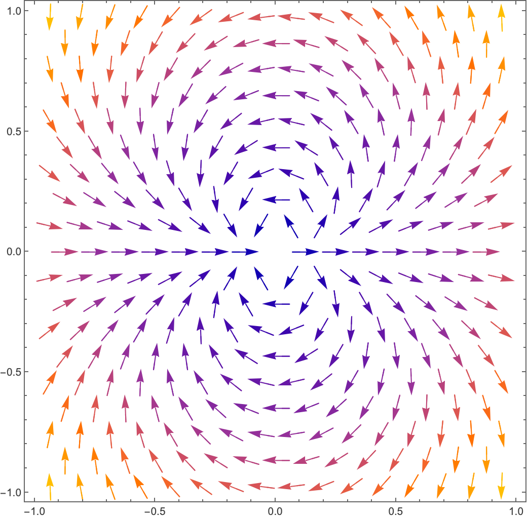
and on inspection we see that the fixed point at the origin has index 2.
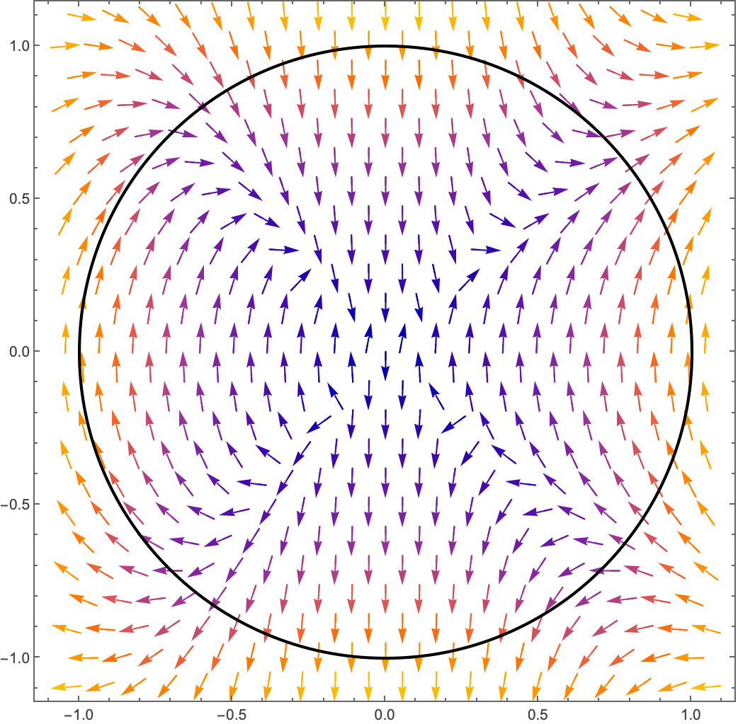
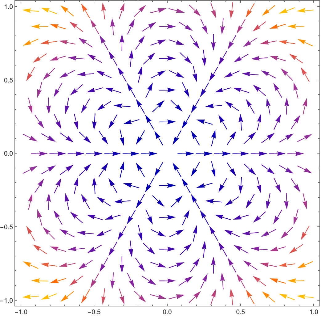
For $n=4 \text{ we have }$
For non-integer values of $n \text{ we end } \text{ up with } $so-called branch-cuts and so the fixed point is no longer isolated so it doesn’t make sense to talk about the index of the fixed point.
Can we get the index from integration in this case?
Let’s look at the case of $n=2$:
$$ \dot{x}=x^{2}-y^{2} $$$$ \dot{y}=2x y $$So we have that
$$ \phi{}=\text{ arctan }\left(\frac{2x y}{x^{2}-y^{2}}\right) $$Let’s convert this to polar coordinates:
$$ \phi{}=\text{ arctan }\left(\frac{2 r \text{ cos }\left(\theta{}\right) r \text{ sin }\left(\theta{}\right)}{r^{2}{\text{ cos }}^{2}\left(\theta{}\right)-r^{2}{\text{ sin }}^{2}\left(\theta{}\right)}\right)=\text{ arctan }\left(\frac{2 \text{ cos }\left(\theta{}\right) \text{ sin }\left(\theta{}\right)}{{\text{ cos }}^{2}\left(\theta{}\right)-{\text{ sin }}^{2}\left(\theta{}\right)}\right)=\text{ arctan }\left( \text{ tan }\left(2\theta{}\right)\right)=2\theta{} $$Integrating this over θ from 0 to 2π tells us that:
$$ I_{C}={\frac{1}{2\pi{}}\left[\phi{}\right]}_{C}=\frac{1}{2\pi{}}{\int{}}_{0}^{2\pi{}}2\theta{}\mathrm{d}\theta{}=2 $$Can we generalise this? Given:
$$ \dot{z}=z^{n} $$We have:
$$ \phi{}=\text{ arctan }\left(\frac{\dot{y}}{\dot{x}}\right)=\text{ arctan }\left(\frac{Im\left(\dot{z}\right)}{Re\left(\dot{z}\right)}\right)=\text{ arctan }\left(\frac{Im\left(z^{n}\right)}{Re\left(z^{n}\right)}\right)=\text{ arctan }\left(\frac{Im\left(r^{n} e^{i n \theta{}}\right)}{Re\left(r^{n} e^{i n \theta{}}\right)}\right)=\text{ arctan }\left(\frac{\text{ sin }\left(n \theta{}\right)}{\text{ cos }\left(n \theta{}\right)}\right)=n \theta{} $$So
$$ I_{C}={\frac{1}{2\pi{}}\left[\phi{}\right]}_{C}=\frac{1}{2\pi{}}{\int{}}_{0}^{2\pi{}}n \theta{}\mathrm{d}\theta{}=n $$