Section 1.5: Reversible systems

Section 1.5: Reversible systems

If you make a movie of an egg dropping on the floor and then play it forwards and backwards, it’s very obvious which one is the correct direction. Eggs don’t simply coalesce from a mess on the floor, and jump back up into your hand.

Well, actually that’s not quite true. In theory, they can, but the chances of them doing this are exponentially small in the number of particles in the system. What would it take for this strange reversal to happen?

Well, you would need that the particles in the floor which are all jiggling around because they have some temperature all happen to jiggle in just the right way to push the bits of egg together at just the right moment. The particles in the egg itself would also all have to be jiggling in just the right way that the energy from them goes into chemical bonds which reform the egg and have enough left over to propel the egg up off the floor. Unlikely, I say, but technically not impossible…although in the lifetime of the universe, even if there were a million cracked eggs on a million floors in every planet in every galaxy in the observable universe, the chances of this happening even once are basically zero, so we say that this process is not reversible.

The paragraph above was really about entropy and the arrow of time, and we ’re not going to go into that now, though there ’s much to be said about it.

How about if I take a video of a pendulum swinging back and forth and play it one way, and then the other way? You won’t be able to tell which one is the ‘correct’ direction, because each behaviour is just as likely. We can say that a pendulum swinging is a reversible system. The dynamics with time running in one direction is equivalent to the dynamics with time running in the other direction.

Let’s say we just take the pendulum starting on the left and swing it one half oscillation to the right. Now if you played the video backward it would look different to if you played the video forward. However, if we reversed both the time, and swapped left for right, the two videos would look exactly the same.

Swapping the direction of time is the same as swapping $t<-> -t$. Let’s look at this more generally, and in terms of the equations themselves.

Let’s go back to our Newton’s law for a conservative system:

$$ m \ddot{x}=F\left(x\right) $$

which is equivalent to:

$$ m \frac{d^{2} x}{d t^{2}}=F\left(x\right) $$

which is really

$$ m \frac{d}{d t}\frac{d}{d t}x=F\left(x\right) $$

The first thing that we see here is that if we let $t\to -t, $then $\frac{d}{d t}\to $ $\frac{d}{d \left(-t\right)}=-\frac{d}{d t}$, and so $\frac{d^{2}}{d t^{2}}\to \frac{d^{2}}{d t^{2}} $ie. it doesn’t change.

So that under the transformation of $t\to -t $the equation of motion remains the same.

Actually we have to be slightly more careful here because we would like to know what’s happening in the phase plane (labeling the phase plane directions $\left(x,v\right)$). So let’s go to the coupled first order system:

$$ \dot{v}=\frac{F\left(x\right)}{m} $$$$ \dot{x}=v $$

Now, if we just let $t\to -t, $then the system doesn’t remain the same. If we just did this then we’d end up with:

$$ -\dot{v}=\frac{F\left(x\right)}{m} $$

$$

• \dot{x}=v $$

which is a different set of equations. If however we also let $v\to -v$ then all of a sudden we get back to

$$ \dot{v}=\frac{F\left(x\right)}{m} $$$$ \dot{x}=v $$

Which says that if we swap the direction of time, and the direction of the velocity then the system remains invariant. This makes sense in terms of the pendulum. Swap the direction of time, and the video will look the same, just with everything moving in the opposite direction.

What does this look like in terms of a trajectory? Well, taking some part of a trajectory in the phase plane, for instance:

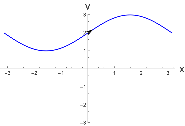
Letting $v\to -v$ will reflect the curve about the x-axis, but we also have to let $t\to -t$ which corresponds to reversing the direction of the arrow to, so this will give the red curve in the figure below:

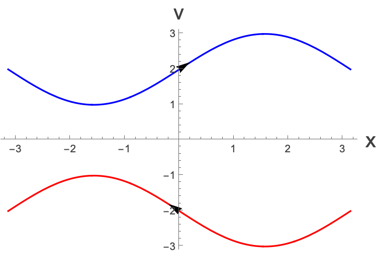
The system is reversible, if the red curve is also a trajectory of the original system.

In terms of the equations, any system for which $t\to -t$ and $v\to -v$ is a symmetry is reversible.

Given a more general system:

$$ \dot{x}=f\left(x,y\right) $$$$ \dot{y}=g\left(x,y\right) $$

what constraints are there on $f$ and $g$ such that the system is reversible under $t\to -t$ and $y\to -y$ (note that we have written $y \text{ now instead } \text{ of } v \text{ to be } a \text{ bit more } \text{ general }.$

Well, first of all performing the transformations we get:

$$

• \dot{x}=f\left(x,-y\right) $$

$$ \dot{y}=g\left(x,-y\right) $$

where the $\dot{y}$ has not changed sign because both $t \text{ and } y $have changed.

So for this to be invariant under the change, we need that $f$ is odd in $y$ and $g \text{ is even } \text{ in } y$ which will give us back our original system.

So that’s it. For a two-dimensional first order system to be reversible (ie. time reversal invariant), we need that $f$ is odd in $y$ and $g \text{ is even } \text{ in } y$.

Remember from the last section that if you take a conservative system, where there is a linear center (ie. when you perform the linear analysis you find a center), then this center is robust in the full non-linear model (ie. the center is really there in the full system, not just the linearised system). Well, it turns out that in reversible systems, the same holds. A center which is really there in the non-linear system is called a non-linear center.

We will state a theorem which will be in terms of a system which has a linear center at the origin of the phase plane. This can be extended to any position along the x-axis of the phase plane.

Essentially this says that if you know that you have the following linear center:

If the system is reversible, then whatever happens near the linear center must form a closed orbit, and must be reflectively symmetric about the x-axis. For instance:

One way to think about this is that the instability of a linear center can lead to a stable or unstable spiral in general. However, if the system is reversible, whatever is happening above the x-axis must be mirrored below the x-axis. This rules out spirals around a linear center and so the orbits about it can only be closed orbits, and not spirals.

Example

Let’s look at

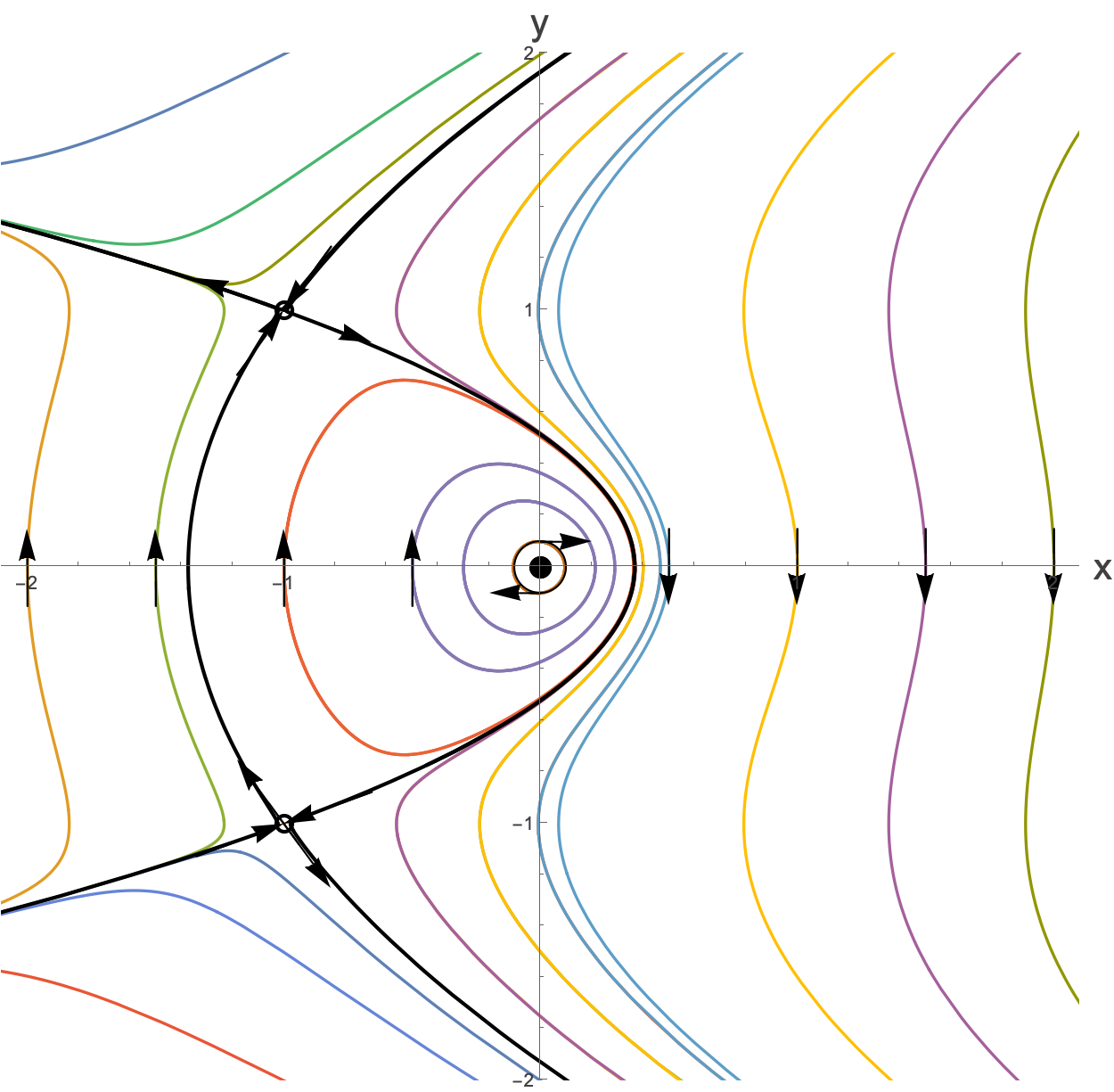
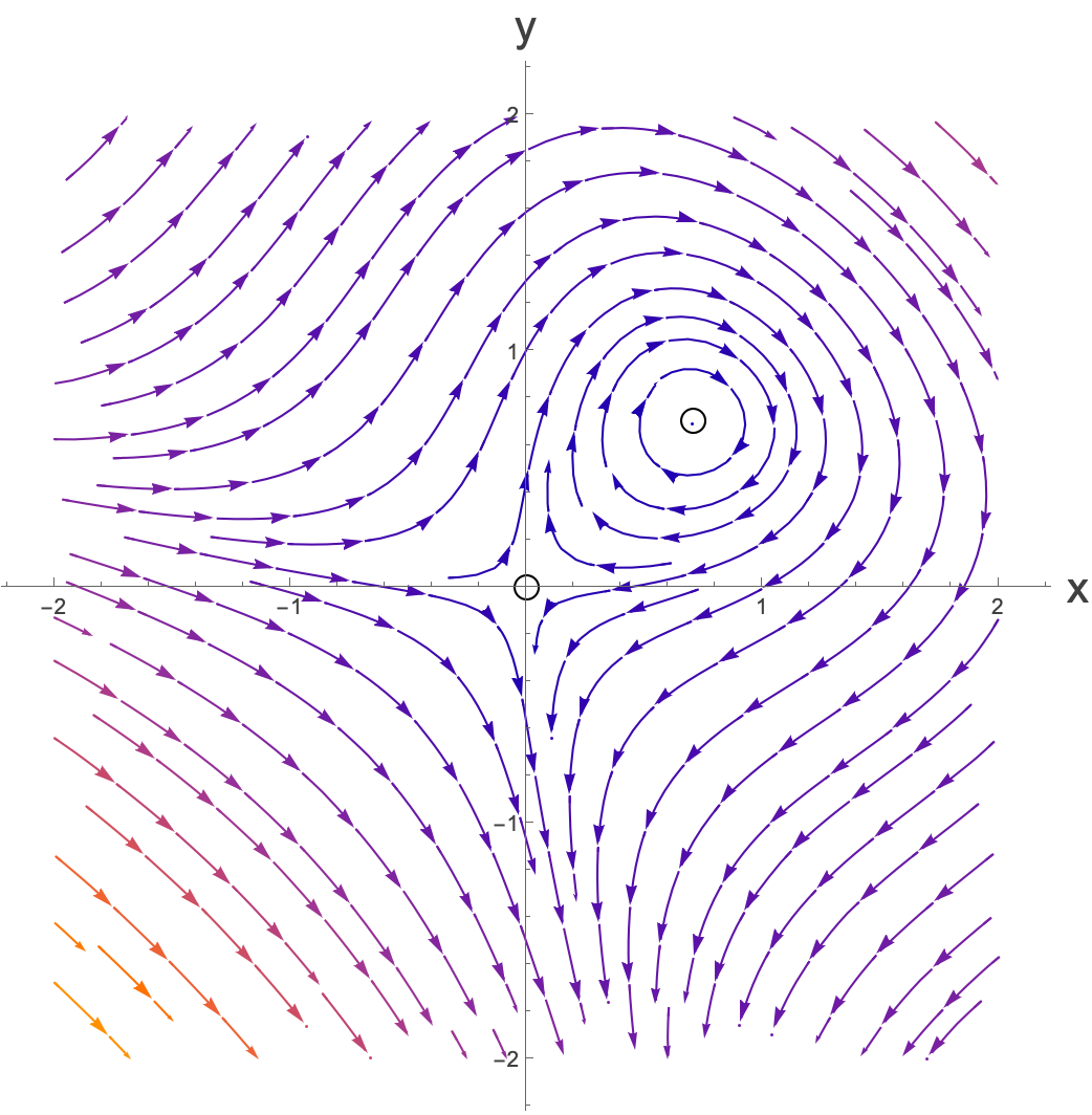
$$ \dot{x}=y-y^{3} $$$$ \dot{y}=-x-y^{2} $$

First we see that the $\dot{x}$ equation is odd in $y$, and the $\dot{y}$ equation is even in $y$, so our system is reversible. We know immediately that it will be symmetric about the x-axis.

Finding the fixed points is equivalent to solving

$$ 0=y-y^{3} $$$$ 0=-x-y^{2} $$

Which has solutions at:

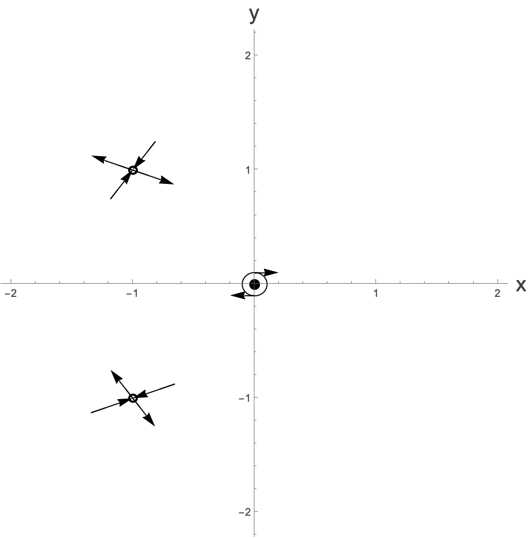
$$ \left(0,0\right), \left(-1,1\right) \text{ and } \left(-1,-1\right) $$

Let’s focus on the fixed point at the origin. The Jacobian of this system is

$$ A=\left(\begin{matrix} 0 & 1-3y^{2} \\ -1 & -2 y \end{matrix}\right) $$

which for the origin is

$$ A_{\text{ origin }}=\left(\begin{matrix} 0 & 1 \\ -1 & 0 \end{matrix}\right) $$

Which sits at the point (1,0) in the $\left(\Delta{},\tau{}\right) \text{ plane and } $so is indeed a center. We can also see that close to the origin, our system linearises to:

$$ \dot{x}=y $$$$ \dot{y}=-x $$

which tells us that the center is moving in the clockwise direction (for $x=0 \text{ and } y=1, \dot{x}$ is positive)

OK, so we have a reversible system, with a center at the origin, so we know that we must have closed cycles around the fixed point at the origin.

For the other fixed points we have

$$ A_{\left(-1,1\right)}=\left(\begin{matrix} 0 & -2 \\ -1 & -2 \end{matrix}\right) , A_{\left(-1,-1\right)}=\left(\begin{matrix} 0 & -2 \\ -1 & 2 \end{matrix}\right) $$

Which are at

$$ \left(-2,-2\right) \text{ and } \left(-2,2\right) $$

respectively. ie. they are both saddle points. We can calculate the eigenvalues and eigenvectors of these Jacobians and we get:

At $\left(-1,1\right)$:

$$ \lambda = -1 - \sqrt{3},\quad \mathbf{v} = \left(-1 + \sqrt{3},\; 1\right) $$$$ \lambda = -1 + \sqrt{3},\quad \mathbf{v} = \left(-1 - \sqrt{3},\; 1\right) $$

At $\left(-1,-1\right)$:

$$ \lambda = 1 + \sqrt{3},\quad \mathbf{v} = \left(1 - \sqrt{3},\; 1\right) $$$$ \lambda = 1 - \sqrt{3},\quad \mathbf{v} = \left(1 + \sqrt{3},\; 1\right) $$

which corresponds to one positive and one negative eigenvalue ($1+\sqrt{3}$ is positive, $1-\sqrt{3}$ is negative) in both cases (unsurprisingly), and we have the associated flow directions for each.

Let’s just focus on the first fixed point’s the eigenvalues and eigenvectors. At (-1,1) we have

$$ {\lambda{}}_{1}=-1-\sqrt{3}, v_{1}=\left(\begin{matrix} -1+\sqrt{3} \\ 1 \end{matrix}\right) $$$$ {\lambda{}}_{2}=-1+\sqrt{3}, v_{2}=\left(\begin{matrix} -1-\sqrt{3} \\ 1 \end{matrix}\right) $$

${\lambda{}}_{1}$ is negative, so this corresponds to the inflowing eigenvector. ${\lambda{}}_{2} \text{ is positive }$ so this corresponds to the outflowing eigenvector.

We can look at the same thing for the fixed point at (-1,-1)

Let’s draw on what we know…

We also know that there are no other fixed points in this system, so there ’s not a great deal of freedom about what the trajectories could be doing. One other piece of information that we do have though is that everything is differentiable, and so we don’t expect any sharp jumps in trajectories, and so because of reversibility, whenever we pass through the x-axis it will be perpendicular to it. This just says that we know that there must be a reflection about the x-axis in the trajectories. In the absence of the smoothness condition, we could have, for instance:

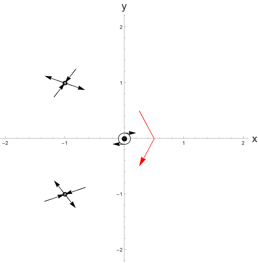
But this has a sudden turn in it on the x-axis. This could only come about because of some discontinuity in the vector field or its derivatives, so anything that passes through the x-axes has to do so orthogonally.

We can figure out the direction by the flows about the fixed points:

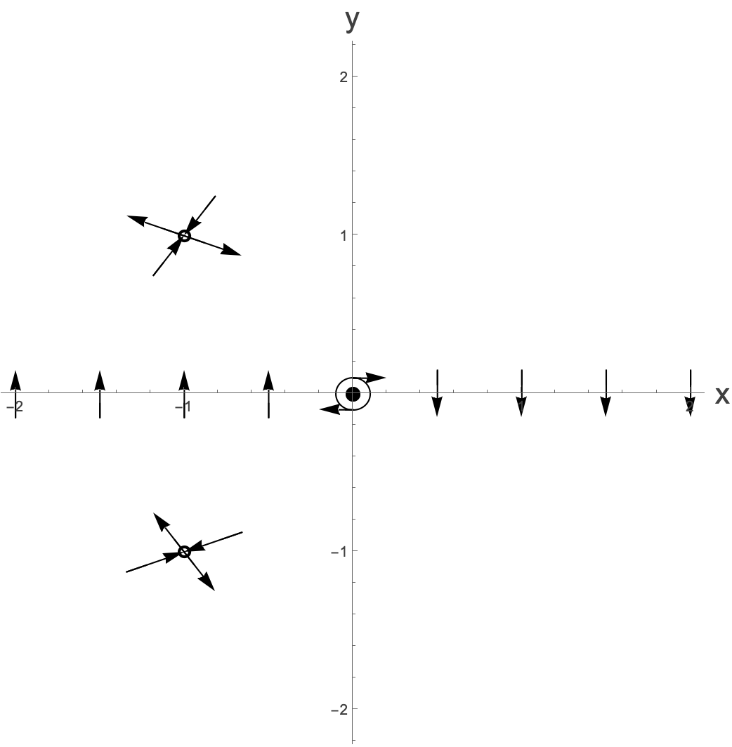
Let’s think about just one trajectory, the one carrying on from this arrow:

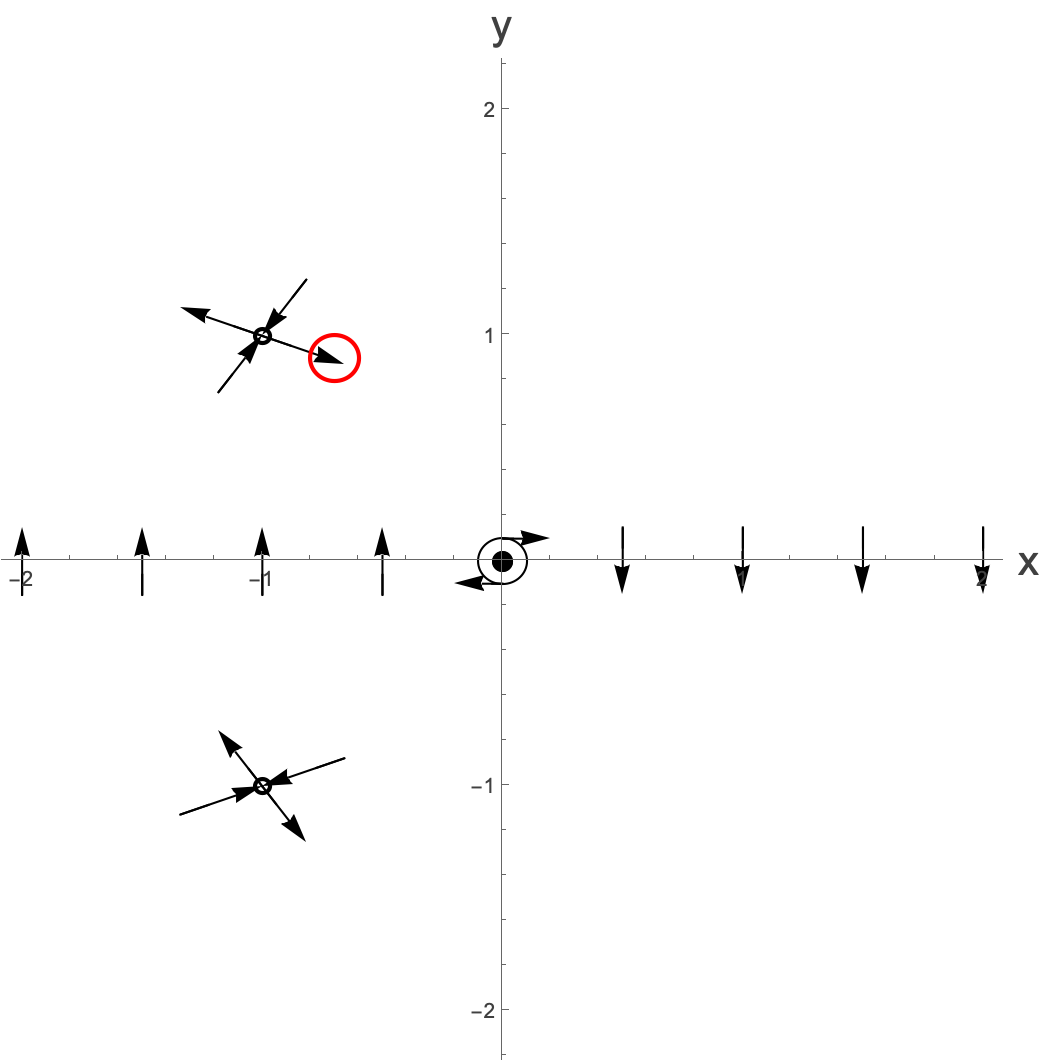
What could it possibly do next given that we know that there are no more fixed points? Well we see that the arrows directly below it are pointing in the opposite direction, so it can’t meet up with them, and the arrows along the positive x-axis are all pointing down, so the only place it could seem to go such that the arrows pointing down can link up with anything would be somewhere on that positive x-axis.

Give it a go and see if you can imagine what the flow might look like.

Well, I’m just going to write down the whole flow for a few trajectories, but you don’t have to know how to do this exactly.

Pretty neat, huh?

While we couldn’t have figured out the precise trajectories of this using our techniques, we could have had a good guess at their qualitative features.

Note that there are two trajectories joining the two saddlepoints, one going to the left of the center, and the other going to the right. These are called heteroclinic trajectories or saddle connections. Note that a homoclinic trajectory starts and ends at the same saddle point and a heteroclinic trajectory links two different saddle points.

Here are plots of the homoclinic (the orange paths on the left) and heteroclinic trajectories (the black paths on the right) for comparison: $$

An important generalisation

We have spoken about the particular time-reversal symmetry of $t\to -t$ along with the equivalent of the reversal in the velocity, but we can actually find systems which are time reversal invariant when we make some other transformation in the (x,y) plane. The only constraint is that whatever the transformation $\left(x,y\right)\to R\left(x,y\right)$, the application of this transformation again has to take us back to (x,y), i.e $R^{2}\left(x,y\right)=\left(x,y\right)$. An example of this used below is of $\left(x,y\right)\to \left(-x,-y\right).$

Are all conservative systems reversible, and vice versa?

For the case of a reversible system which is not conservative. See exercise 2 below.

For the case of conservative systems which are not reversible, I was able to find a couple of papers which discuss this in the literature, though the systems are a lot more complicated than we cover in this course. These papers are:

Take a look if you want to know more.

Can we find a reversible system where there is a centre which is not on the x-axis?

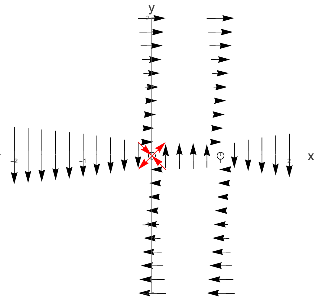
We start with a system where the centre is on the x-axis, but not at the origin. This is given by

$$ \dot{x}=y $$$$ \dot{y}=x-x^{2} $$

We can see that a) this system has the right symmetries to be reversible ($f\left(x,y\right)$ is odd in $y$ and $g\left(x,y\right)$ is even in $y$). We can see that there are two fixed points in this system, at (0,0) and (0,1). We can show that these correspond in the linearisation to a saddle, and a center. Saddles are robust to nonlinearities, and so it will still be a saddle. The centre will also be robust, because this system is reversible. We can get a good picture of what is going on simply by plotting the flows at the null-clines, and plotting the direction of flow as well as the eigenvector directions for the saddle (in red):

Taking the red arrows, there’s only really one thing that they can do:

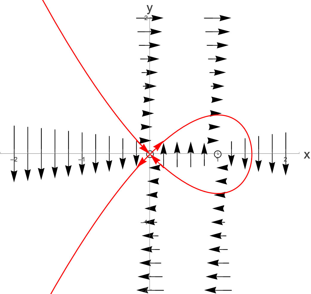
Plotting the flow lines on top of this we get:

So we see that we have a homoclinic orbit. OK, but we just have a system which is reversible and has a center on the x-axis. How could we turn this into something with a center away from the x-axis. Well, remember that for a reversible system, actually we just need that we have a symmetry such that under some $R$, we have that $R^{2}\left(x,y\right)=\left(x,y\right)$ and $t\to -t$. This is any reflection, and so we can actually rotate the whole plane, and there will still be a reflection symmetry.

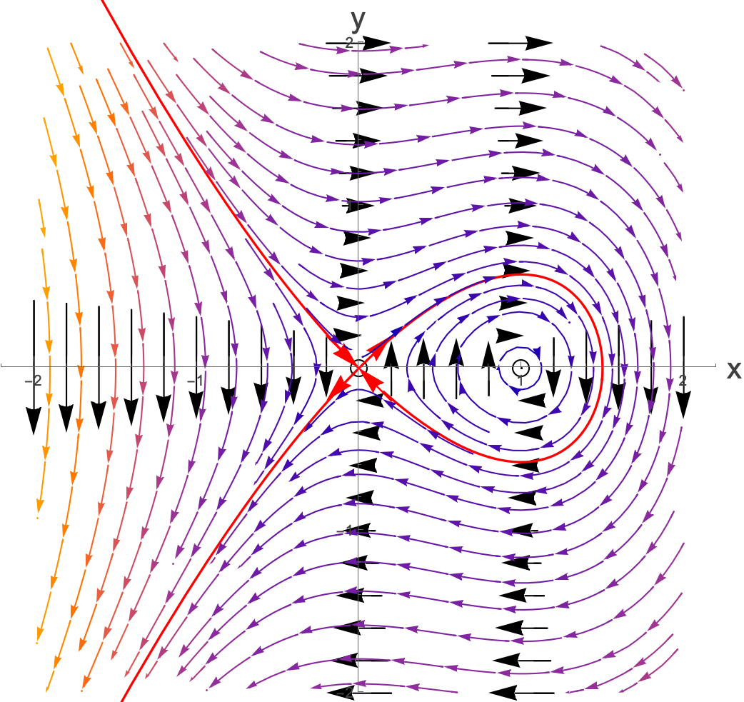
Let’s rotate the coordinate system by -$\frac{\pi{}}{4} \text{ radians in } \text{ the anticlockwise } \text{ direction } $which will be equivalent to rotating the system by $\frac{\pi{}}{4}$ anticlockwise. To do this we can perform a rotation on our $\left(x,y\right) $coordinates as:

$$ \left(\begin{matrix} x' \\ y' \end{matrix}\right)=\left(\begin{matrix} \text{ cos }\left(-\frac{\pi{}}{4}\right) & -\text{ sin }\left(-\frac{\pi{}}{4}\right) \\ \text{ sin }\left(-\frac{\pi{}}{4}\right) & \text{ cos }\left(-\frac{\pi{}}{4}\right) \end{matrix}\right) \left(\begin{matrix} x \\ y \end{matrix}\right)=\frac{1}{\sqrt{2}}\left(\begin{matrix} 1 & 1 \\ -1 & 1 \end{matrix}\right) \left(\begin{matrix} x \\ y \end{matrix}\right) $$

Performing this change of variables and then just relabelling the new $x'$ and $y'$ to $x \text{ and } y$ gives:

$$ \dot{x}=\frac{1}{4}\left(-4 x+\sqrt{2} x^{2}+2 \sqrt{2} x y+\sqrt{2} y^{2}\right) $$$$ \dot{y}=\frac{1}{4} \left(-\sqrt{2} x^{2}+4 y-2 \sqrt{2} x y-\sqrt{2} y^{2}\right) $$

This looks like a hell of a mess, but if you now plot the flow lines in this new system we see:

We see that there is a reflection symmetry about the line $y=x$ and thus the system is reversible and we have a fixed point away from the $x-\text{ axis }.$

An exercises for you

1. Given

$$ \dot{x}=-2 \text{ cos } x-\text{ cos } y $$$$ \dot{y}=-2 \text{ cos } y-\text{ cos } x $$

Sketch the phase portrait.

Note that this has an attracting fixed point, and so cannot be conservative, but it can be reversible. Check whether this is true.

Assignment

The non-dimensionalised pendulum is modelled by

$$ \ddot{\theta{}}+\text{ sin } \theta{}=0 $$

1. Write this as a coupled set of first order equations.

2. Is the system reversible?

3. Is the system conservative? Find the energy as a function of the phase space coordinates.

3. Calculate the fixed points of the system

4. Calculate the Jacobian at the fixed points. You should find that there are two unique Jacobians for the infinite number of fixed points. Why is this?

5. What sort of fixed points are they?

6. What does reversibility and conservation of energy tell you about the nature of one of the linear fixed points?

7. By finding the eigenvalues and eigenvectors of the Jacobian, plot the trajectories close to the three closest fixed points to the origin in phase space.

8. Use the energy function to plot some characteristic trajectories above and below the horizontal axis.

9. For $E=1$ you should find heteroclinic orbits. Indicate these in the diagram.

10. What dynamics do the saddles correspond to?

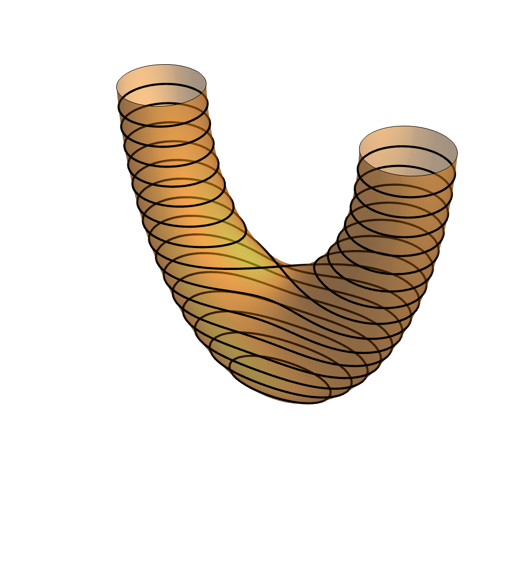
11. The phase plane as you have it is infinitely long in the $\theta{}-\text{ direction }$. Cut the phase plane at the first left and first right saddle points to the center, and imagine folding this up into a cylinder, identifying the two saddle points and standing the cylinder on its end. Try and sketch what trajectories would look like.

12. This one is tricky to visualise! You can take the cylinder that you have, and rather than plotting the angle and angular velocity directions, plot the angle around the cylinder and the energy vertically. You should end up with something that looks like this. You are NOT expected to be able to figure this out for yourself. However, I want you to spend a while pondering what this means. Ignore the gaps in the lines…this is just a function of the way that this is plotted.

13. Extension: Now imagine that you add a damping term to this system. Is it still conservative? Is it still reversible? How will the phase space look now? Try and draw the phase space just by thinking about the behaviour of a damped pendulum and without going through all of the calculation. What would the equivalent of the strange u-shaped diagram above look like for the damped trajectories?