Section 1.4: Conservative systems

Section 1.4: Conservative systems

We are going to just touch the surface of one of the most important topics in modern physics - that of conservation laws. I’m sure that you’ve all heard of the conservation of energy, but this is just one particular example of a conservative quantity. Conservation laws are related to symmetry properties of a system, and understanding symmetries leads to a deep understanding of many different types of system. In particular, within much of theoretical high energy physics, symmetry is at the heart of, well, almost everything.

Emmy Noether was the mathematician who really elucidated the connection between conservation laws and symmetries and Noether’s theorem is still used every day by thousands of physicists around the world.

Unknown author. Publisher: Mathematical Association of America, Brooklyn Museum, Agnes Scott College - Emmy Noether (1882-1935), Archived

In terms of the conservation of energy, this is actually linked to a symmetry called time translational invariance. Essentially this means that the system is invariant with respect to the time that you look at it at.

If you are doing an experiment in a laboratory where there are windows, you may find that your system is not time translationally invariant, because it might matter whether you’re doing it in the day or night, because heat conducts through the windows at a different rate at different times. You would find that your system does not necessarily conserve energy.

However, if you closed all the doors and put blinds on the windows then maybe your system would be time translationally invariant. If you have very very sensitive equipment however, then the gravitational pull of the sun and the earth may make a difference which would again break this symmetry.

Anyway, we will not worry about the details of this too much now, but that ’s just a quick taster as to the importance of symmetries. For now, we are going to be interested in particular types of conservative systems.

Let’s start off with a second order system given by Newton ’s law

$$ m \ddot{x}=F\left(x\right) $$

You can also write this as $F=m a. $Here $m \text{ is the } \text{ mass }$ of some object and it says that the acceleration of the object is equal to the force applied to it divided by the mass. Small masses accelerate faster under a given force than do large masses.

Note that we have written here that the force can be a function of the position, but not of time (corresponding to a driving force), or of the velocity of the object (corresponding to a damping force)

We can rewrite the above by defining a potential energy $V\left(x\right)$ whose derivative is the negative of the force:

$$ F\left(x\right)=-\frac{d V}{d x} $$

This says that the force comes from a difference in the potential energy between two points. The reason you accelerate under gravity is because the potential energy at different vertical heights is different, and so there is a gradient in the potential energy which means that there is a force on you which means that you accelerate.

It turns out that for all systems for which $F \text{ is } $a function only of $x$ you can write the force in terms of this gradient.

We can now write Newton’s law as

$$ m \ddot{x}+\frac{d V}{d x}=0 $$

Now multiply both sides by $\dot{x}$:

$$ \dot{x} m \ddot{x}+\dot{x} \frac{d V}{d x}=0 $$

Show that this is the same as writing

$$ \frac{d}{d t}\left(\frac{1}{2}m{\dot{x}}^{2}+V\right)=0 $$

where we have used the chain rule, noting that really $V=V\left(x\left(t\right)\right)$.

We say that the left hand side is an exact time-derivative. Exact here meaning that the terms on the left can be written as the time derivative of the simple expression in brackets.

In fact the thing in brackets is the kinetic energy plus the potential energy, which generically is the total energy, which we can call $E:$

$$ E=\frac{1}{2}m{\dot{x}}^{2}+V $$

So

$$ \frac{d E}{d t}=0 $$

This equation is exceptionally important. This says that the energy of the system will not change over time. What that means in practice is that for a given trajectory in phase space, the energy will always remain the same.

Although in this case it was the energy which is conserved, there are many different types of quantity that can be conserved, and this generically means that for a quantity $Q$ to be conserved

$$ \frac{d Q}{d t}=0 $$

along trajectories in phase space and that $Q$ is a real-valued function and is nonconstant on every open set.

Addition to the previous version of the notes: Why do we require that it has to be nonconstant on every open set? Well, this is because for ANY dynamical system, a fixed number is constant on every open set. Let’s say that I choose the function Q=5 for all x. Well, we could, naively say “hooray, we ’ve found a conserved quantity, therefore there can ’t be any nodes or spirals”. But this is a trivial case and doesn’t put any constraint on the path. Sure, numbers are always constant, but that doesn’t give any constraint on the dynamics, which non-trivial Q does.

If we had an attracting fixed point in a system, then all trajectories in the basin of attraction would lead to that fixed point, and so if we had a conservative system, all of those trajectories would have the same conserved quantity (let’s call it energy for now), and so everywhere in the open set around the fixed point would have the same constant energy and so the above conditions would not hold. Of course, even in this case, there is a trivial conserved quantity, which is just any constant function, but that doesn’t tell us anything interesting.

Here we see an attracting fixed point. If we had energy conservation in this system then every trajectory would have to have the same energy as that at the fixed point, and so they would all have to have the same energy and so everything in this region would have to have the same energy and so you wouldn’t have a non-constant energy in that open set.

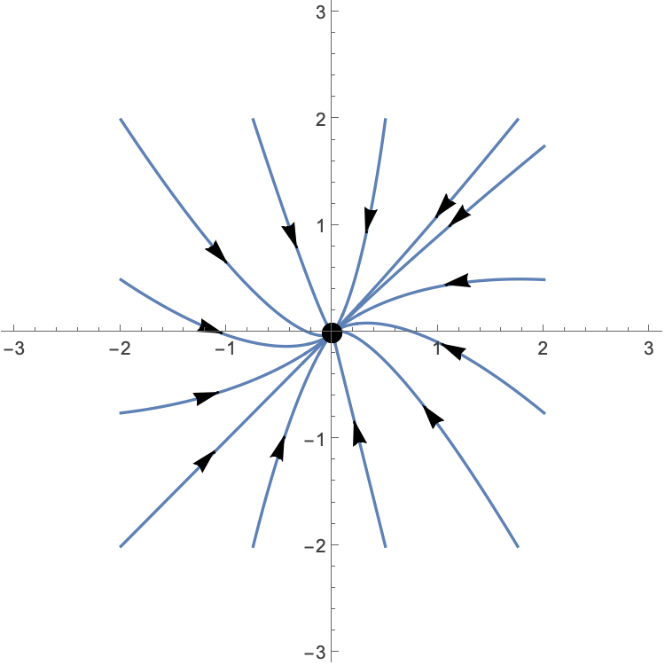
This tells us that we cannot have any attracting fixed points in a conservative system (one for which there exists a conserved quantity). However, one can have saddles and centers in conservative systems.

Let’s look at an example of this. In fact this is going to be the first example that we looked at in this course, but we will go into it in more detail now.

A double-well potential is a potential which has…two wells. For instance:

$$ V=-\frac{1}{2}x^{2}+\frac{1}{4}x^{4} $$

looks like:

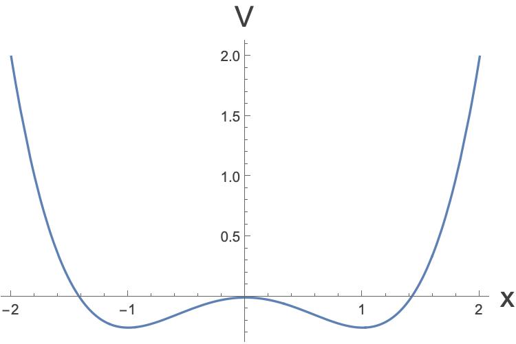
Remember that the force is equal to the negative of the gradient, so where there is a steep gradient, the force is larger and at the bottom of the two wells there is zero gradient so no force and the particle just sits there.

Writing Newton’s law for this system and fixing $m=1$) gives:

$$ \ddot{x}+\frac{d \left(-\frac{1}{2}x^{2}+\frac{1}{4}x^{4}\right)}{d x}=0 $$$$ \ddot{x}=x-x^{3} $$

We can use the old trick that we learned in MAM1043H to write this second order system as two first order systems:

$$ \dot{x}=y $$$$ \dot{y}=x-x^{3} $$

Make sure that you can show that there are three fixed points: ${\text{ fp }}_{1}\text{ at }$ $\left(-1,0\right), {\text{ fp }}_{2}\text{ at } \left(0,0\right), {\text{ fp }}_{3} \text{ at } \left(1,0\right).$

The Jacobian of this system is:

$$ A=\left(\begin{matrix} 0 & 1 \\ 1-3x^{2} & 0 \end{matrix}\right) $$

Which at the three fixed points gives

$$ A_{1}=\left(\begin{matrix} 0 & 1 \\ -2 & 0 \end{matrix}\right), A_{2}=\left(\begin{matrix} 0 & 1 \\ 1 & 0 \end{matrix}\right), A_{3}=\left(\begin{matrix} 0 & 1 \\ -2 & 0 \end{matrix}\right) $$

Leading to:

$$ \left({\Delta{}}_{1},{\tau{}}_{1}\right)=\left(2,0\right), \left({\Delta{}}_{1},{\tau{}}_{1}\right)=\left(-1,0\right), \left({\Delta{}}_{1},{\tau{}}_{1}\right)=\left(2,0\right) $$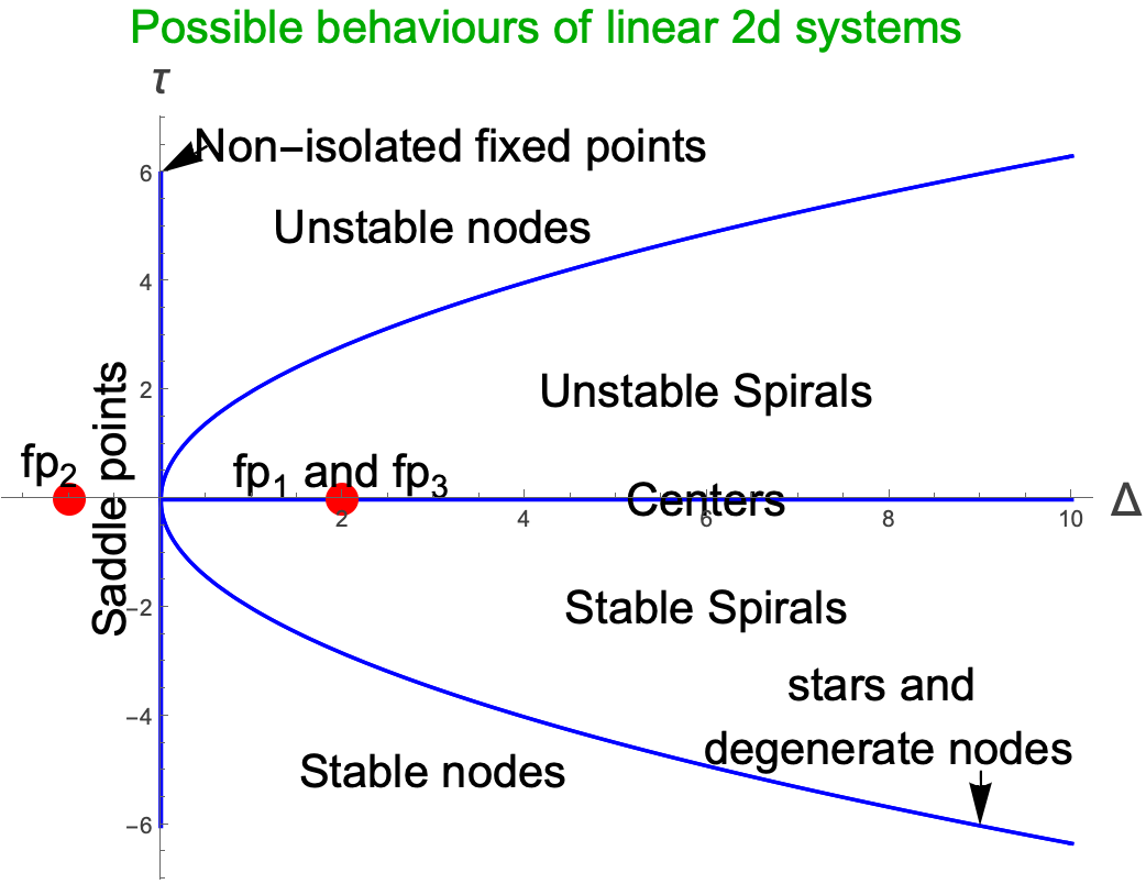

So we have two centers and one saddle point.

What do we remember from the section about linearisation? That centers are very very sensitive to non-linearities, and what might look like a center when we linearise might become either an attracting or repelling fixed point when we include non-linearities. So perhaps those centers are just a linearised dream and if you looked at the whole system they would disappear.

However, we also know that our system is conservative and so there can ’t be any stable or unstable spirals or stars or degenerate nodes (attracting or repelling fixed points), so somehow the center may still remain.

In fact we can find the trajectories by finding the paths for which $E$ is a constant. $E \text{ in this } \text{ case }$ is just (remembering that $m=1\right)$:

$$ E=\frac{1}{2}{\dot{x}}^{2}+V $$$$ =\frac{1}{2}y^{2}-\frac{1}{2}x^{2}+\frac{1}{4}x^{4} $$

So if we can plot out the contours for which

$$ \frac{1}{2}y^{2}-\frac{1}{2}x^{2}+\frac{1}{4}x^{4}=\text{ constant } $$

we have found our trajectories. In other words:

$$ y=\pm{}\sqrt{2\text{ constant }+x^{2}-\frac{1}{2}x^{4}} $$

where the constant is of course the energy, so:

$$ y=\pm{}\sqrt{2E+x^{2}-\frac{1}{2}x^{4}} $$

Let’s first look at a large positive value of $E$, say $E=1$.

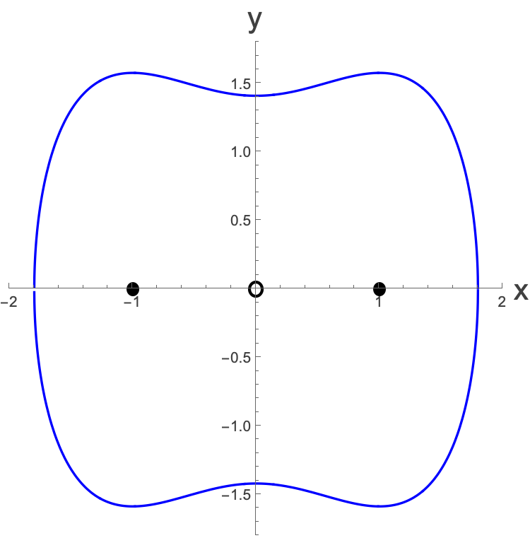
What do we have here? Well, first of all we should figure out what direction we would travel around the trajectory. Well, let’s look at the point around $\left(0,1.42\right)$, right at the top. If we plug that into the equations then we get:

$$ \dot{x}=1 $$$$ \dot{y}=0 $$

So $x \text{ is increasing } \text{ at this } \text{ point and } \text{ so } $the trajectory must be going clockwise:

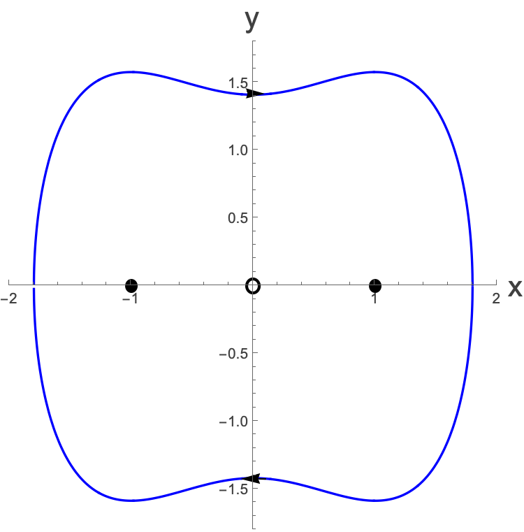
So what does this mean? Well, this trajectory corresponds to the system moving from around $x=-1.8 \text{ to } x=1.8 \text{ and back } \text{ again over } \text{ and over }$. However, the (absolute) y-value (which is actually |$\dot{ x}$|, ie. the speed) is smallest at the extremes of $x$, then gets larger, then smaller for a bit at $x=0$, then larger again.

Looking at our potential again:

This is a trajectory that looks like:

Where we are thinking of the potential as a gravitational potential being proportional to the height. Because there is no friction in the system, the particle will roll about forever exchanging potential energy for kinetic energy and back again.

OK, let’s look at this first for small negative values of $E$, say $E=-0.1$ (don’t worry about negative energies here):

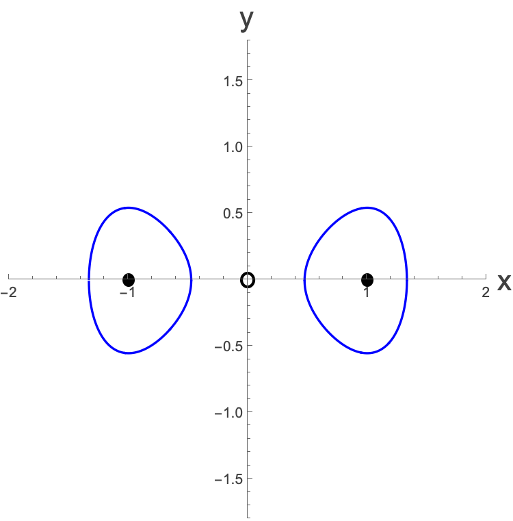
What is going on here? Well, again we can calculate the direction of the arrows. Make sure that you can see that this must be:

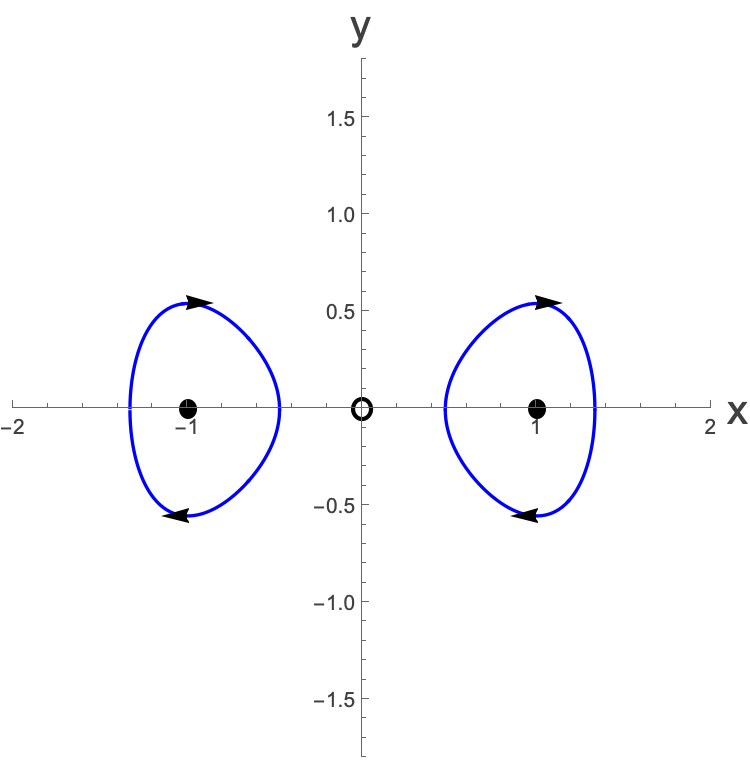
This corresponds to trajectories which are stuck in one of the wells - either the left well or the right well. They can never escape.

It definitely looks here like the energy of this solution is less than that of the one that goes between both wells.

So let’s stop dilly-dallying about and put in a load of different trajectories of different energies:

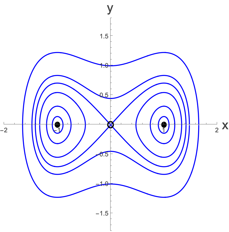
We see one trajectory which ‘crosses through’ the saddlepoint (it never actually crosses it, because you can’t pass over a saddlepoint). In fact this is the zero energy trajectory. It has just enough energy to get to the top of the peak in the middle, but it takes forever to get there. Plotting one of the very very nearby trajectories looks like this:

Now putting everything together with all the appropriate arrows we end up with the same plot that we had back in section 1.1:

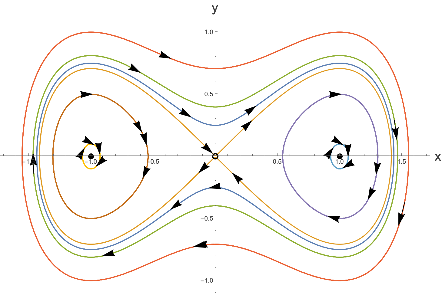
The yellow orbits which starts from the saddle point and ends at it are known as a homoclinic orbits. In this case every orbit is periodic apart from the two homoclinic orbits. You never quite get to the saddle point, and if you start from exactly the saddle point, it’s a bit like the Hotel California.

We can actually do a better visualisation than this. Remember each trajectory corresponds to a constant energy. Well, how about we do this in a 3d plot where the height is the energy of that trajectory:

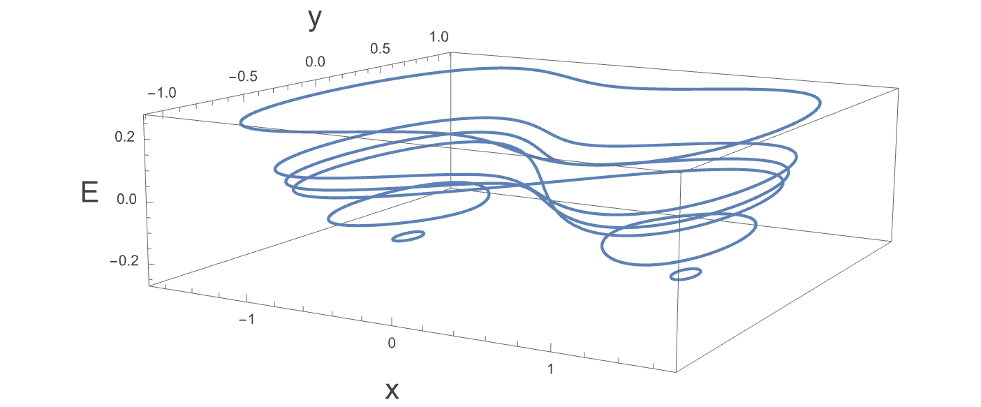
Looking at this as a surface plot is simply the energy function that we wrote down before:

$$ E =\frac{1}{2}y^{2}-\frac{1}{2}x^{2}+\frac{1}{4}x^{4} $$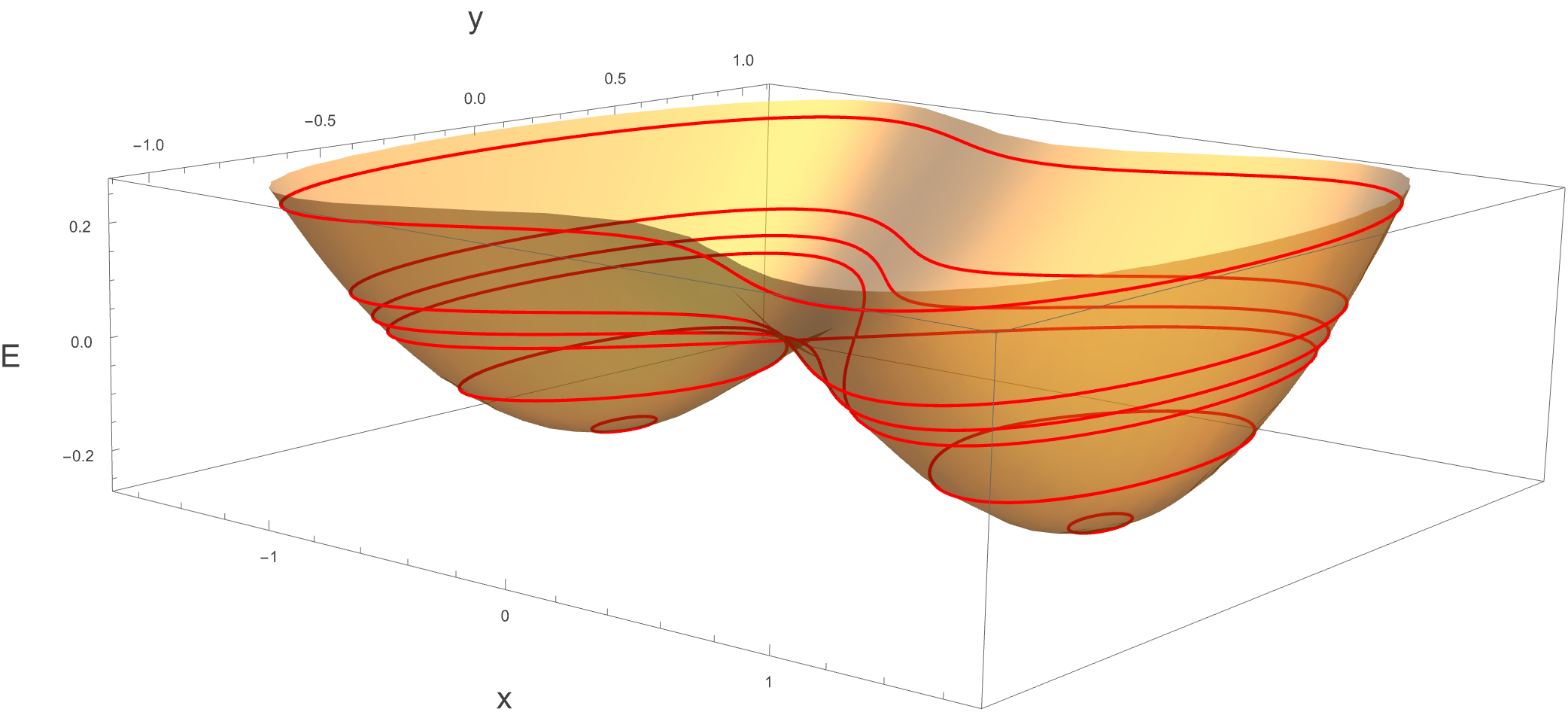

This is a plot of the energy function of this system. Keep in mind as always that y is really the velocity. So we take the system at any position and any velocity and it will tell us the energy of the system for all time to come after that as it traces one of the contours on the energy surface.

One important thing to note here is that the dynamics of this system shouldn ’t be confused with the dynamics of the particle rolling about in the double well. Dynamics here all happens along horizontal cross-sections corresponding to energy contours.

A projection of these contours into the $\left(x,y\right) \text{ plane simply } \text{ gives the } \text{ trajectories in } \text{ the phase } \text{ space }.$

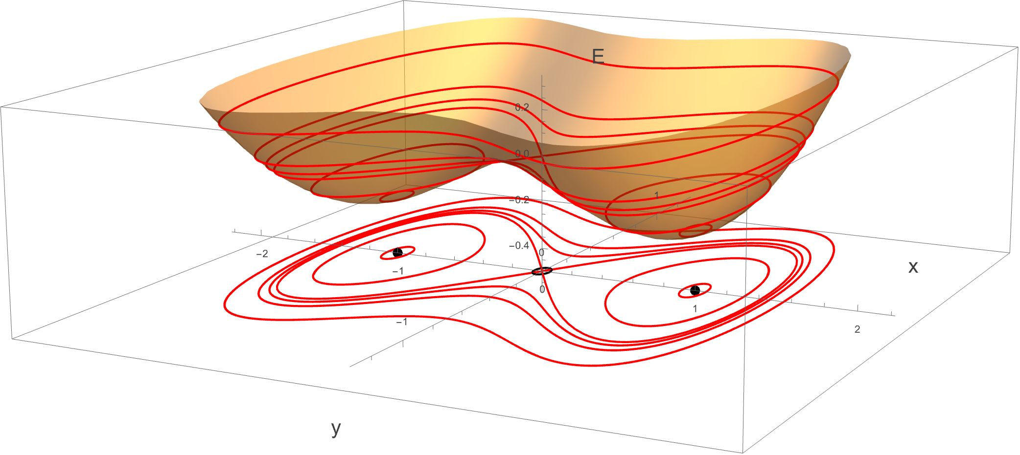
Note that in this case the centers correspond to the minimal energy solutions and are stable fixed points. This won’t always be the case, but you would have to come up with non-differentiable potentials to find such scenarios, so we won’t worry about them here.

Remember that we performed our fixed point analysis by looking at the Jacobian at the fixed points. This is equivalent to linearising the system, and we said that centers are very unstable to non-linearities…but it looks like the old centers are still centers, even if they don’t correspond to perfect circles, or ellipses. Why is this?

Well, this is a special feature of conservative systems and corresponds to a general theorem about such systems:

Given a general two-dimensional dynamical system, where the dynamics is governed by a continuously differentiable set of functions, the variables $\left(x,y\right)\in{}$ $R^{2}$, and there exists a conserved quantity $E\left(x,y\right)$. If there is an isolated fixed point which is a local minimum (or maximum) of $E\left(x,y\right) \text{ then }$ all trajectories sufficiently close to the fixed point must be closed cycles.

We won’t prove this theorem, but you should think about why this might be by looking at the energy surface, the centers and the local minima in the example we’ve been going through here.

Try and think what happens also if the fixed point is not isolated - for instance if we had a line of fixed points…would this hold?

Hang on, but I thought that conservative vector fields were curl free?

So, there are two things which shouldn’t be conflated here. A conservative system in the sense of there being conservation of energy, and a conservative vector field in the sense that around any closed curve there is no work done on the particle. In the latter case, the vector field is the force on the particle and thus you should think of this as a system, maybe in two dimensions, with forces acting on it. Here we are really thinking about a system which lives in a two dimensional phase space, but the ‘spatial’ location is just one dimensional. When we are talking about a vector field in this course we mean a vector field in phase space and this is different from having something of the form:

$$ F=\nabla{}\phi{} $$

Which is a conservative vector field, which is indeed curl free.

Essentially “conservative” here has two different meanings. In our case, there can be curl in the vector field in the phase plane.

Assignment 2

We’re going to look here at an equation which comes from general relativity. It’s going to be a bit strange to start with, as where we normally expect time, we’re actually going to see a different variable.

Let’s imagine that we have a planet orbiting a star. We can write the coordinates in polar coordinates and we could think of writing $r\left(t\right) \text{ and } \theta{}\left(t\right)$ as the positions in the plane of motion. However, it’s possible to do a change of variable which allows us to think not about the motion through time, but the trajectory in a sort of parametric way, where we have r(θ). As an example, if you wrote an equation

$$ r\left(\theta{}\right)=\theta{} $$

This would correspond to a spiral. as θ increases, so $r$ increases.

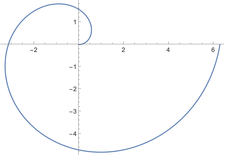
We could plot something more complicated, like

$$ r\left(\theta{}\right)=\text{ sin }\left({\theta{}}^{2}\right)+\frac{1}{1+{\theta{}}^{2}} $$

I’ve no idea what this looks like…let ’s see…

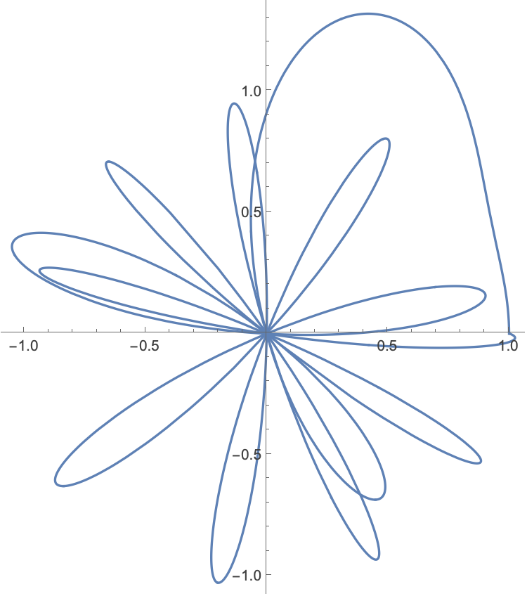
Gahhh! That’s kinda cool…

OK, so it turns out that you can write the equations in General Relativity for a planet moving about a star in a differential equation in terms of r( θ)…but we’re going to mess things up a bit and instead define $u=\frac{1}{r}$ and write things in terms of u(θ). Drumroll…

$$ \frac{d^{2}u}{d {\theta{}}^{2}}+u=\alpha{}+\epsilon{} u^{2} $$

where α comes out of classical gravity and is a positive parameter, and ε $u^{2}$ is the so called relativistic correction. We can think of ε as a very small parameter which tells us that the real world is well approximated by classical gravity, but that we need to take relativity into account if we want really precise answers.

You should look at this equation, and see how it compares with Newton ’s law (hint hint):

$$ \frac{d^{2}x}{d t^{2}}=\frac{-d V}{d x} $$

OK, so we can also take the equation for u(θ) and do our usual trick to turn it into two first order equations…actually, that’s a lie…you can!

1. Letting $v=\frac{d u}{d \theta{}}$ write the equation as a system in the $\left(u,v\right) \text{ plane }.$

2. Find the equilibrium points of the system and classify them using linear stability analysis.

3. If you found a center, you now want to show that this is in fact a non-linear center. How would we do this? Well, we know that if there is a conserved quantity in the system, then a linear center will remain a center. We have to be a bit careful here as we’re not looking for some quantity $E\left(u,v\right)$ for which:

$$ \frac{d E\left(u,v\right)}{d t}=0 $$

there’s no $t$ floating about. You need to find a quantity for which

$$ \frac{d E\left(u,v\right)}{d \theta{}}=0 $$

where remember $u \text{ and } v \text{ are functions } \text{ of } \theta{}.$

a) Use the lessons learned in this chapter to find such a quantity.

• b) Show that it is indeed conserved.

• c) Show that the linear center you found (which you now know is a non-linear center) is a minimum of $E \text{ and not } $a maximum. To do this, you need to do the equivalent of calculating the second derivative and showing that it’s positive for it to be a local minimum. This is done using the Jacobian, but not the same Jacobian that you’ve been looking at so far in this course. Calculate:

$$ \left(\begin{matrix} \frac{{\partial{}}^{2}E}{\partial{}u^{2}} & \frac{{\partial{}}^{2}E}{\partial{}v\partial{}u} \\ \frac{{\partial{}}^{2}E}{\partial{}u\partial{}v} & \frac{{\partial{}}^{2}E}{\partial{}v^{2}} \end{matrix}\right) $$

And calculating the determinant of this. So long as $\frac{\partial{}E}{\partial{}u} \text{ and } \frac{\partial{}E}{\partial{}v} $are both zero, if the determinant of the Jacobian is positive then you are at a local minimum.

4. This equilibrium point corresponds to a circular orbit. Show this, and find what its radius is.