Section 1.3: Fixed Points and Linearisation

Section 1.3: Fixed Points and Linearisation

Again we had a look at this topic back in MAM1043H. If you don ’t remember this in detail (or at all), take a look here. Note also that I’ve added a very small section at the end in blue here which I had not discussed last year and will be important for the assignment.

It’s going to turn out that most of the time, the ideas about being able to linearise about fixed points to study stability will hold in two dimensions. Some of the time however the linearised system is in the class of “borderline” cases of Centers, Stars, Degenerate Nodes and Non-isolated Fixed Points. In these cases we have to be a little more careful as funny things can happen as we will see below.

But we’re getting ahead of ourselves here. Let ’s just see how we can extend the ideas of linearising a one-dimensional system to linearising a two-dimensional one.

We start, as always these days, with our system looking like:

$$ \dot{x}=f\left(x,y\right) $$$$ \dot{y}=g\left(x,y\right) $$

where $f \text{ and } g \text{ are } $any non-linear functions, although we will require them to be differentiable at the fixed points. We will also presume that we have found a fixed point, at $\left(x^{*},y^{*}\right)$ in the phase plane. Similar to the one-dimensional case, we will write our functions $x \text{ and } y$ as:

$$ x\left(t\right)=x^{*}+u\left(t\right) $$$$ y\left(t\right)=y^{*}+v\left(t\right) $$

where now $u \text{ and } v \text{ are the } \text{ dynamical parts }$ which are essentially telling us about movement around the fixed point. The idea is going to be that we will ask what happens when $u \text{ and } v \text{ are }$ both small, ie. when $x \text{ and } y \text{ are }$ close to their fixed point values. We will call $u \text{ and } v $the components of a disturbance from the fixed point. Let’s just look at an intuitive example of this.

Let’s say that we have a particle moving about in a bowl, where the bowl is given by the equations

$$ h={\left(x-2\right)}^{2}+{\left(y+3\right)}^{2} $$

This looks like

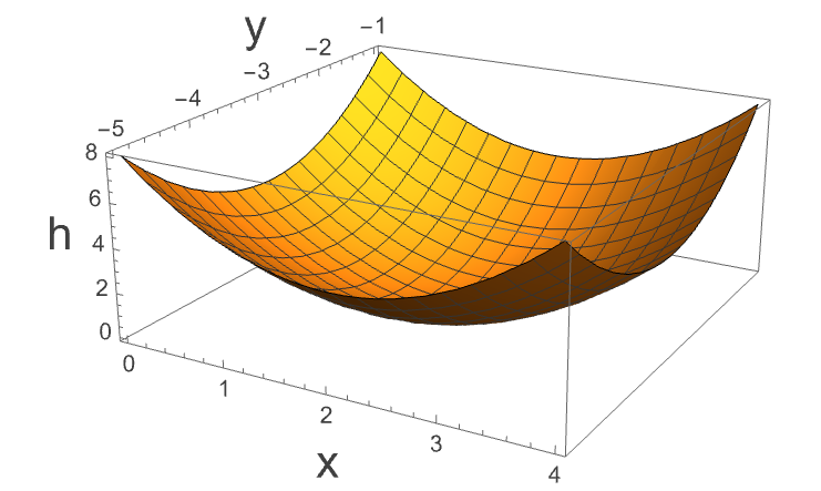
We could describe the position of the particle in terms of $x$ and $y_{ } \text{ positions }$, but we know that in this case the ‘fixed point ’ is at $\left(2,-3\right), \text{ so if } \text{ we define } x=2+u, y=-3+v, $then we can describe the movement in terms of $\left(u,v\right) \text{ coordinates }$, and now if $u \text{ and } v \text{ are both } \text{ small }, \text{ then we } \text{ are close } \text{ to the } \text{ fixed point } \text{ of this } \text{ system }, \text{ and }$ could study these small perturbations if we wished.

Anyway, this is just a toy example. Let’s think about things more generally.

Remember that in the one dimensional example, we were able to write $\dot{x}=f\left(x\right) \text{ as } \dot{u}=f\left(x^{*}+u\right)=f\left(x^{*}\right)+u\frac{d f\left(x\right)}{\text{ dx }}|_{x^{*}}+...$ Well, now we are going to do the same thing, but this time in two variables. We start by writing:

$$ \dot{u}=f\left(x^{*}+u,y^{*}+v\right) $$$$ \dot{v}=g\left(x^{*}+u,y^{*}+v\right) $$

where we have been able to write $\dot{x}={\dot{x}}^{*}+\dot{u}=\dot{u}$ because $x^{*} \text{ is } $a constant and therefore its time derivative is zero…and similarly for $v$. Now let’s take the first of these expressions and perform a Taylor expansion about $\left(x^{*},y^{*}\right)$:

$$ \dot{u}=f\left(x^{*}+u,y^{*}+v\right) $$$$ =f\left(x^{*},y^{*}\right)+u{\partial{}}_{x}f\left(x,y\right)|_{x^{*},y^{*}}+v{\partial{}}_{y}f\left(x,y\right)|_{x^{*},y^{*}}+\mathcal{O}\left(u^{2},v^{2},u v\right) $$

ok, so some notation here ${\partial{}}_{x}f\left(x,y\right)$ is just the partial derivative of $f$ with respect to $x$ and we are then evaluating this at the fixed point. $\mathcal{O}\left(u^{2},v^{2},u v\right)$ says that we are neglecting terms of order $u^{2},v^{2} \text{ and } u v$ and of course higher order in $u \text{ and } v$. However, because we have said that we are looking at behaviour close to the fixed point, $u^{ }\text{ and } v $are both small, so the higher order terms can be neglected. Performing the same expansion for the second equation we end up with the following two linearised equations (neglecting quadratic terms) in the “disturbance”:

$$ \dot{u}=f\left(x^{*},y^{*}\right)+u{\partial{}}_{x}f\left(x,y\right)|_{x^{*},y^{*}}+v{\partial{}}_{y}f\left(x,y\right)|_{x^{*},y^{*}} $$$$ \dot{v}=g\left(x^{*},y^{*}\right)+u{\partial{}}_{x}g\left(x,y\right)|_{x^{*},y^{*}}+v{\partial{}}_{y}g\left(x,y\right)|_{x^{*},y^{*}} $$

Actually, we can simplify this because we know that at the fixed point, $f \text{ and } g$ both evaluate to zero by definition, so we really have:

$$ \dot{u}=u{\partial{}}_{x}f\left(x,y\right)|_{x^{*},y^{*}}+v{\partial{}}_{y}f\left(x,y\right)|_{x^{*},y^{*}} $$$$ \dot{v}=u{\partial{}}_{x}g\left(x,y\right)|_{x^{*},y^{*}}+v{\partial{}}_{y}g\left(x,y\right)|_{x^{*},y^{*}} $$

We can actually write this whole thing in matrix form as

$$ \left(\begin{matrix} \dot{u} \\ \dot{v} \end{matrix}\right)=\left(\begin{matrix} {\partial{}}_{x}f & {\partial{}}_{y}f \\ {\partial{}}_{x}g & {\partial{}}_{y}g \end{matrix}\right)|_{x^{*},y^{*}}\left(\begin{matrix} u \\ v \end{matrix}\right) $$

The matrix:

$$ A=\left(\begin{matrix} {\partial{}}_{x}f & {\partial{}}_{y}f \\ {\partial{}}_{x}g & {\partial{}}_{y}g \end{matrix}\right)|_{x^{*},y^{*}} $$

Is known as the Jacobian matrix at the fixed point. Jacobians show up all over applied mathematics, and you can see a nice Khan academy video about it here.

This all feels a bit abstract at the moment. Let’s look at a particular example. Taking the two-dimensional non-linear system given by

$$ \dot{x}=-x+x^{3} $$$$ \dot{y}=-2y $$

The first thing that we see is that this system is decoupled. This means that the dynamics in the $x \text{ direction is } \text{ not dependent } \text{ on the } y \text{ position }, \text{ and vice } \text{ versa }. $We could actually find the solutions for $x$ and $y$ separately, but let’s go through the analysis above.

First we want to find the fixed points. These are given by solving $\dot{x}$=$\dot{y}=0.$ and we get three fixed points, at coordinate $\left(-1,0\right),\left(0,0\right) \text{ and } \left(1,0\right)$. We we are trying to do with the linearisation analysis is to get an idea of the nature of these fixed points.

Next we want to find the Jacobian matrix which is the matrix of partial derivatives. Then we will find the Jacobian matrix at the fixed points. This gives us

$$ A=\left(\begin{matrix} -1+3x^{2} & 0 \\ 0 & -2 \end{matrix}\right)|_{x^{*},y^{*}} $$

which, when evaluated at the three fixed points is:

$$ A_{1}=\left(\begin{matrix} 2 & 0 \\ 0 & -2 \end{matrix}\right), A_{2}=\left(\begin{matrix} -1 & 0 \\ 0 & -2 \end{matrix}\right), A_{3}=\left(\begin{matrix} 2 & 0 \\ 0 & -2 \end{matrix}\right) $$

where we have written $A_{i}, i=1,2,3$ for the three fixed points listed above. Now we have the linearised dynamical system where the equations are just:

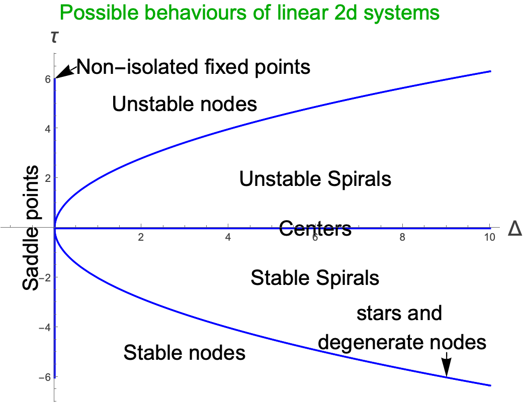
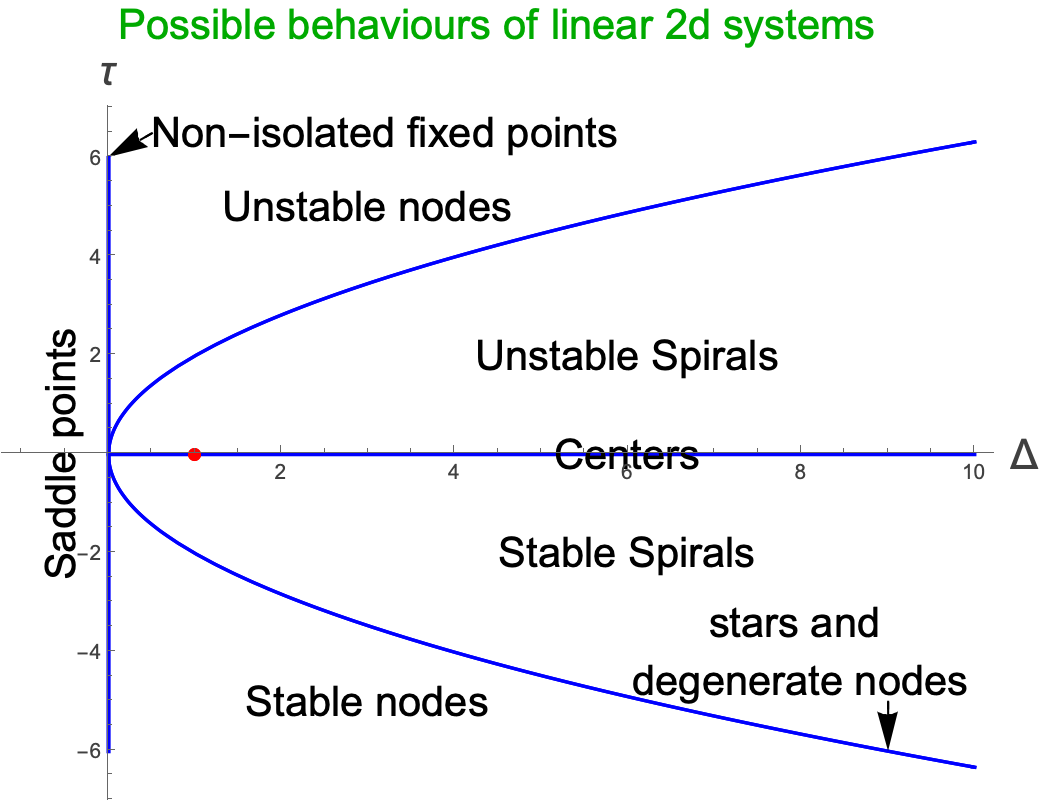
$$ \left(\begin{matrix} \dot{u} \\ \dot{v} \end{matrix}\right)=\left(\begin{matrix} 2 & 0 \\ 0 & -2 \end{matrix}\right)\left(\begin{matrix} u \\ v \end{matrix}\right) \left(\text{ for the } \text{ first and } \text{ last fixed } \text{ points }\right) \text{ and } \left(\begin{matrix} \dot{u} \\ \dot{v} \end{matrix}\right)=\left(\begin{matrix} -1 & 0 \\ 0 & -2 \end{matrix}\right)\left(\begin{matrix} u \\ v \end{matrix}\right) \text{ for the } \text{ middle one }. $$

ok, so now we can deal with these in the same way as we did for any linear second order system. We calculate the trace and determinant and figure out where these lie in the family of different linear second order systems. Make sure that you can see why they sit at the red points in the plot below:

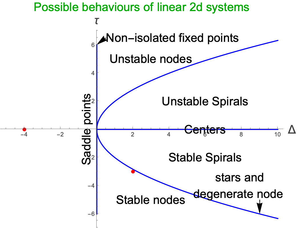
We see here that we have two saddle points (both at the same position in the $\left(\Delta{},\tau{}\right) \text{ plane },$ and one stable node (although it’s close to being a star or degenerate node). Both of these are not the borderline cases that we hinted about above, so we can believe that the linearised system does give us useful information about the full non-linear system in the region close to the fixed points.

Let’s solve the linearised system exactly for the case of

$$ \left(\begin{matrix} \dot{u} \\ \dot{v} \end{matrix}\right)=\left(\begin{matrix} 2 & 0 \\ 0 & -2 \end{matrix}\right)\left(\begin{matrix} u \\ v \end{matrix}\right) $$

This solution to this is:

$$ u=u_{0}e^{2t}, v=v_{0}e^{-2t} $$

So we can write that close to the fixed point at (-1,0) we have:

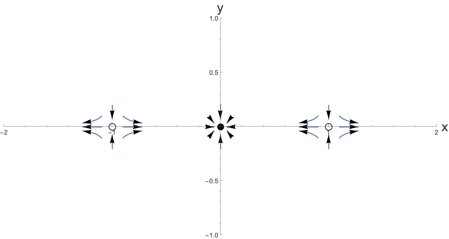
$$ x=-1+u_{0}e^{2t}, y=v_{0}e^{-2t} $$

Plotting some characteristic flows near the fixed point (ie. for small $u \text{ and } v\right)$ we have:

Now doing the same thing for the other fixed points and including the nature of the fixed points we have:

What we have been able to do here is to get a sense of what is happening in this system close to the fixed points.

We can also look at the nullclines. Let’s ask when the flows are perfectly vertical. That would be when $\dot{x}$=0. This is equivalent to solving just

$$ 0=-x+x^{3} $$

but leaving $y$ unfixed. In fact we see here that for $x=-1,0 \text{ and } 1$, the flows are purely vertical. We can then solve for the y equation for these values. Actually, in this case because the system is uncoupled, the value of $x$ has makes no difference and we just have:

$$ \dot{y}=-2y \longrightarrow{} y=y_{0}e^{-2t} $$

which says that these nullclines all correspond to decaying values of $y$. Let’s add these to the phase diagram:

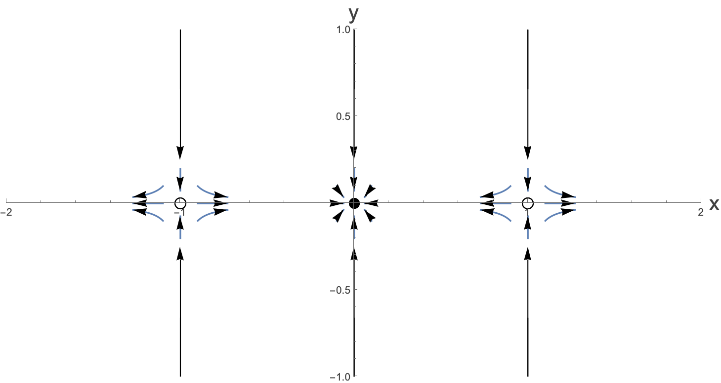
Now for the horizontal nullclines, these are found by setting $\dot{y}=0$, which is solved for $y=0. $We can actually see from the above phase diagram how these lines must flow along the x-axis:

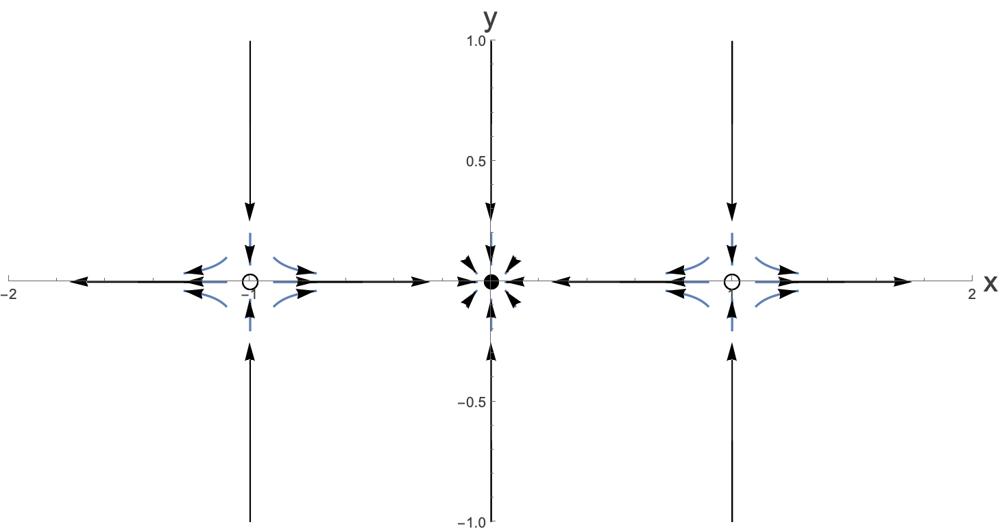
This already gives us a pretty good idea about the flows. Now imagine that you start at the position of the red dot in the following:

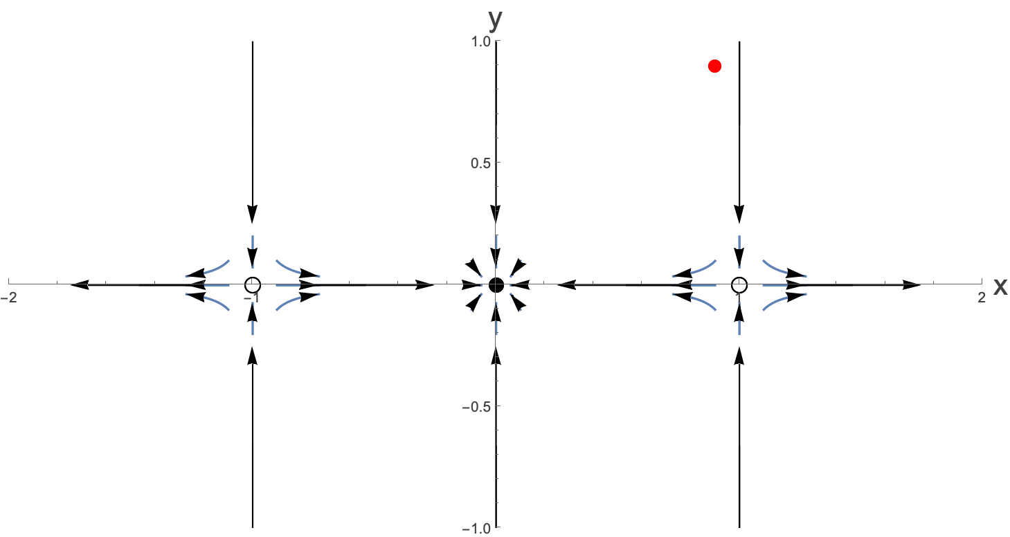
What might the flow of this look like? Well, it looks like it ’s going to mostly move down, but then as it gets closer to the x-axis it’s going to be moving to the left, attracted by the stable fixed point. Indeed solving the system exactly and this flow we see that our intuition is correct:

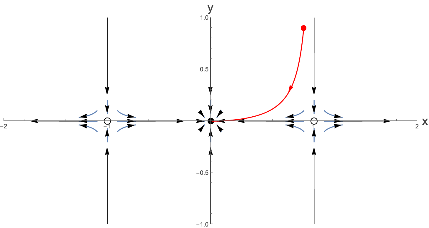
See if you can figure out a way to calculate the red line yourselves.

Doing the same thing at some different initial points we get:

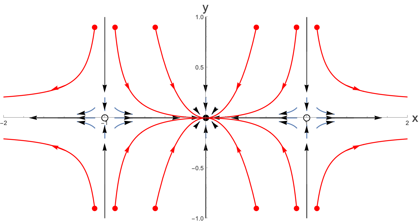
OK, let’s take stock of what we did here. We started off by finding the fixed points of our system. We then linearised around the fixed points and found that the linearised system was not in any of the borderline cases. We plotted some of the trajectories close to the fixed points as well as the nullclines and then used our imaginations to think what the possible flows away from these ones might be. We could then fill in some of the other trajectories by using direction fields, or the Runge-Kutta method.

Next we are going to look at an example where, naively we would have a “Center” solution, but in fact even a tiny non-linearity changes this. Let’s see…

This is actually a carefully chosen example because it can be solved exactly by performing a change of coordinates. We will study the system given by:

$$ \dot{x}=-y+a x \left(x^{2}+y^{2}\right) $$$$ \dot{y}=x+a y \left(x^{2}+y^{2}\right) $$

There is only one fixed point for this system at $\left(x^{*},y^{*}\right)=\left(0,0\right)$. Because of this, dealing with small perturbations is equivalent to dealing with small $x$ and $y$.

I leave it as an exercise for you to see that you can linearise this system about the fixed point as:

$$ \dot{x}=-y $$$$ \dot{y}=x $$

Which can be written as:

$$ \left(\begin{matrix} \dot{x} \\ \dot{y} \end{matrix}\right)=\left(\begin{matrix} 0 & -1 \\ 1 & 0 \end{matrix}\right)\left(\begin{matrix} x \\ y \end{matrix}\right) $$

Which sits here (the red spot) in the space of possible linear systems:

The linearised system can be solved exactly and gives:

$$ x=x_{0}\text{ cos } t-y_{0} \text{ sin } t $$$$ y=x_{0}\text{ sin } t+y_{0} \text{ cos } t $$

which are indeed spirals. For $a=0, \text{ these }$ solutions are exact, and we might imagine that for small $a \text{ they would }$ also be good approximations of the true solutions for small values of $\left(x,y\right)$ and therefore that all solutions would look something like:

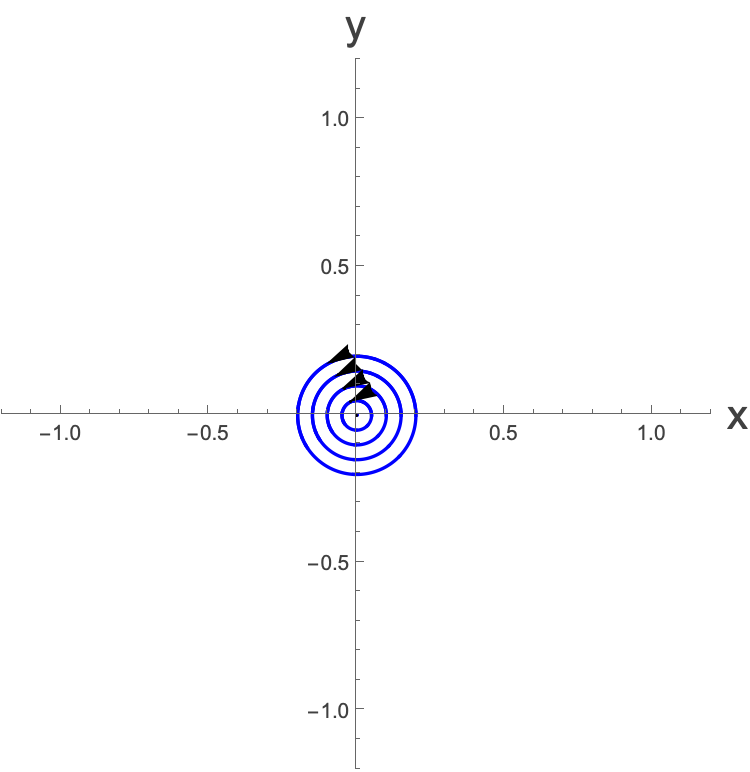
In this small region. However, we can show that this isn’t the case by making a change of coordinates and solving the system exactly.

Let’s go from Cartesian to Polar coordinates by letting $x=r \text{ cos } \theta{}, y=r \text{ sin } \theta{}$ which means that:

$$ \dot{x}=\frac{d \left(r \text{ cos } \theta{}\right)}{\text{ dt }}=\dot{r} \text{ cos } \theta{}-r \dot{\theta{}} \text{ sin } \theta{} $$$$ \dot{y}=\frac{d \left(r \text{ sin } \theta{}\right)}{\text{ dt }}=\dot{r} \text{ sin } \theta{}+r \dot{\theta{}} \text{ cos } \theta{} $$

So we have:

$$ \dot{r} \text{ cos } \theta{}-r \dot{\theta{}} \text{ sin } \theta{} = -r \text{ sin } \theta{}+a r^{3} \text{ cos } \theta{} $$$$ \dot{r} \text{ sin } \theta{}+r \dot{\theta{}} \text{ cos } \theta{} = r \text{ cos } \theta{}+a r^{3} \text{ sin } \theta{} $$

Multiplying the top equation by cos θ and the bottom by sin θ gives us:

$$ \dot{r} {\text{ cos }}^{2} \theta{}-r \dot{\theta{}} \text{ sin } \theta{} \text{ cos } \theta{}= -r \text{ sin } \theta{} \text{ cos } \theta{}+a r^{3} {\text{ cos }}^{2} \theta{} $$$$ \dot{r} {\text{ sin }}^{2} \theta{}+r \dot{\theta{}} \text{ sin } \theta{} \text{ cos } \theta{}= r \text{ sin } \theta{} \text{ cos } \theta{}+a r^{3} {\text{ sin }}^{2} \theta{} $$

Adding the equations together gives:

$$ \dot{r} = a r^{3} $$

Plugging this back into either equation leaves us with:

$$ \dot{\theta{}} =1 $$

So, it would have been easier to start with this, wouldn’t it? Well, the reason that we didn’t was to show (as you ’ll see in a moment) that linearising doesn’t always work.

So, we can solve this exactly and we get:

$$ r =\frac{r_{0}}{\sqrt{1-2 a {r_{0}}^{2} t}}, \theta{}={\theta{}}_{0}+t $$

For $a=0, \text{ indeed we } DO \text{ get } $a circle, as we would expect, because the $a$ is the coefficient of the non-linear element of the equations. However, for $a\neq{}0$ the behaviour is distinctly different. For positive $a$ we can see that as $t \text{ increases }$, $r$ is going to increase, and as $t\to \frac{1}{2a {r_{0}}^{2}}$, $r\to \infty{}$. Conversely, for negative a we see that as $t\to \infty{}$, $r\to 0$. So we will have the following exact solutions:

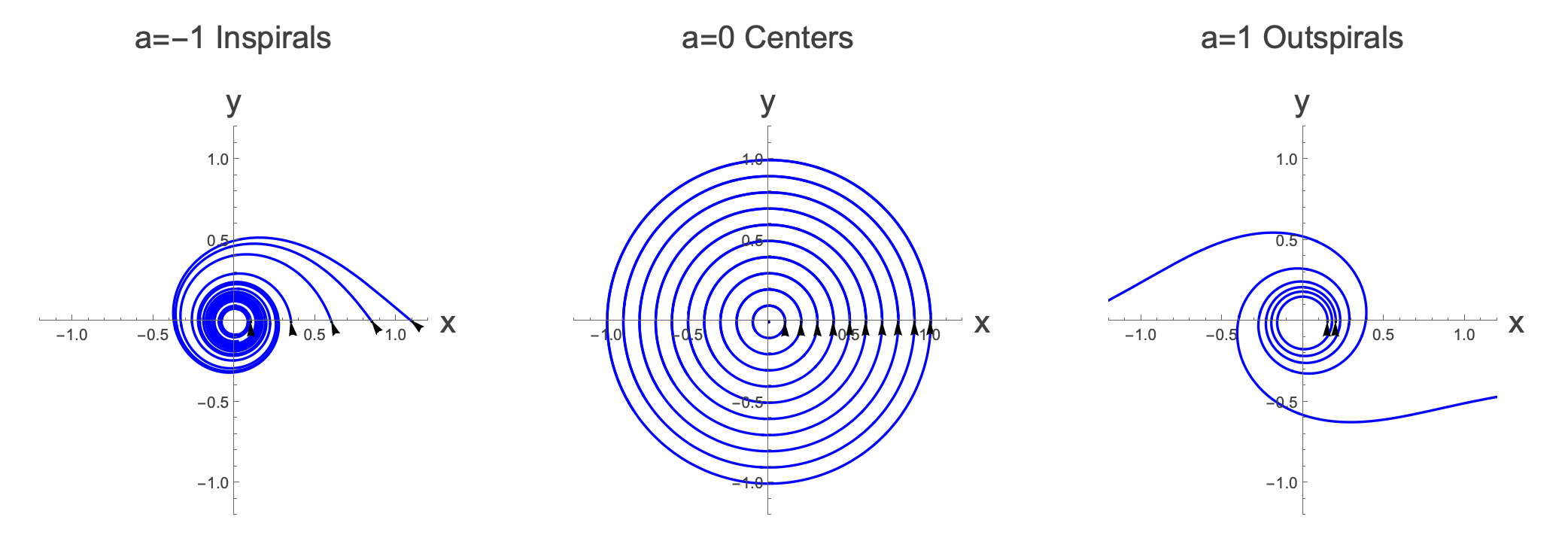
So why is this system so sensitive to any change in $a? Well$, for $a=0 \text{ we have } \text{ perfect center } $solutions. A tiny tiny perturbation from a center solution is going to mean that after one orbit, if the path doesn’t close then we no longer have a center solution and we end up with either an inspiral or outspiral. The solutions would have to change in a very specific way to be perturbed away from centers, and yet to still come back to their starting places after one orbit. This isn’t impossible to imagine, but it’s clearly got to be a very special perturbation to do this.

One thing to note here is that for $a=0$, the fixed point is stable, whereas for $a>0$ it becomes unstable, so the non-linearity can not only change behaviour near the fixed point, it can even change the nature of the fixed point.

So how about the other borderline behaviours, ie. the stars, degenerate nodes and the non-isolated fixed points?

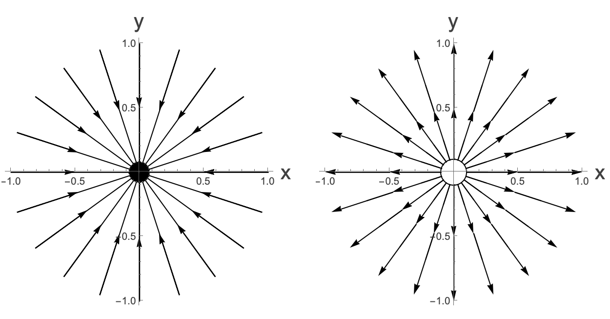
Well, one of the other types was a star, here is a stable and unstable star solution.

We can take a non-linear system, linearise it and find that this corresponds to a star solution. However, the star solution may not remain and one might get an inspiral or outspiral again. However, importantly the nature of the fixed point will not change. Adding a non-linearity will not change a stable to an unstable fixed point or vice versa.

Similarly stable and non-stable degenerate node where there is a single real repeated eigenvalue where there is one uniquely determined eigenvalue, and the other eigenvalue is undetermined.

Here is an example of a stable degenerate node:

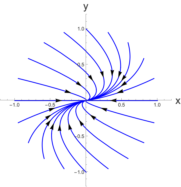
Again, if we alter this by a non-linearity, we won’t change the nature of the fixed point, but it can change the system so that the number of eigenvectors can change and so a stable degenerate node can become a stable node or stable spiral and an unstable degenerate node can become and unstable node or an unstable spiral. This makes sense looking at the diagram once more:

Similarly non-isolated fixed points (fixed points along a whole line, or, in the extreme case where everything is a fixed point) can be altered to become all of the non-boundary cases. It should be clear from looking at this plot that centers are the only ones on the boundary between stable and unstable, so depending on the particular non-linearity, they may become stable or unstable, whereas the other boundary types won’t change the nature of the fixed point.

We can figure out which of the different cases are robust (the nature of the fixed points doesn’t change when the system is perturbed away from non-linearity) and marginal (where the nature of the fixed point can change) by looking at the eigenvalues.

It is the real part of the eigenvalues which tells you whether you are going to be attracted to or repelled from the fixed point. If both eigenvalues are real and positive, you have a repeller. If both are real and negative you have an attractor, and if both are real, with one positive, and one negative, then you have a saddle-point. Adding in a non-linearity won’t change the sign for points close to the fixed point, so the nature of these won’t change, as the only thing it can do is to shift the magnitude of the eigenvalues and possibly add an imaginary part. However the imaginary part just tells you about whether you have angular motion around the fixed point and not its nature. All of these cases are robust. These cases where there is a non-zero real part to both eigenvalues are called hyperbolic cases.

If however you have both eigenvalues purely imaginary, then a tiny deformation from non-linearity can add a tiny real part which alters the nature of the fixed point completely. Similarly, if one of the eigenvalues is zero, then again, a tiny change can alter the stability completely. All of these cases are marginal.

The Hartman-Grobman theorem:

The statement about hyperbolic solutions being robust is a general statement that can be made for systems in any number of dimensions. It can be shown that of you have a system of n-nonlinear differential equations, and if the linearised system, about some fixed point is hyperbolic (all eigenvalues have a real part), then the local trajectories close to a hyperbolic fixed point is topologically equivalentto the linearisation about the fixed point.

This topological equivalence means that you can make a continuous and invertible transformation of the paths in the phase space between the linearised and non-linear system in such a way that the arrow of time remains the same.

Robust/hyperbolic systems are also called structurally stable. A small perturbation will make a small change to the behaviour of the system. Marginal/non-hyperbolic systems are structurally unstable. A small change can make a big difference!

See here for a lovely discussion about these ideas:

What if we can’t linearise?

Remember in the first year course, where we looked at linearising systems, and found that for some, linearising didn’t work. For instance, if you try and linearise:

$$ \dot{x}=x^{2} $$

Then naively you will simply find that close to the fixed point at $x=0:$

$$ \dot{x}=0 $$

But the solution to this is $x=x_{0}$ which clearly doesn’t make sense, as that says that close to the fixed point, solutions are all fixed points. The point is that with linearisation, we can only throw away higher order terms if they are less important than lower order terms. And here there are no lower order terms.

In everything that we’ve spoken about above, it would seem that we can always linearise, but we can’t always trust the linearisation when we are on one of the boundary solutions. However, this isn ’t always true. For instance, given:

$$ \dot{x}=y-x $$$$ \dot{y}=x^{2} $$

If we naively try to linearise about the fixed point at $\left(x,y\right)=\left(0,0\right)$, we would find that the Jacobian is

$$ A|_{x^{*},y^{*}}=\left(\begin{matrix} -1 & 1 \\ 0 & 0 \end{matrix}\right) $$

which has Δ=0, τ=-1, and we would classify this as having non-isolated fixed points…which doesn’t make sense as we know that the fixed point is at (0,0). We’ve lost vital information by getting rid of the $x^{2} $part. The issue is that we simply can’t linearise this equation. It is what it is, and the fixed point doesn’t have any interpretation in terms of the linear fixed points.

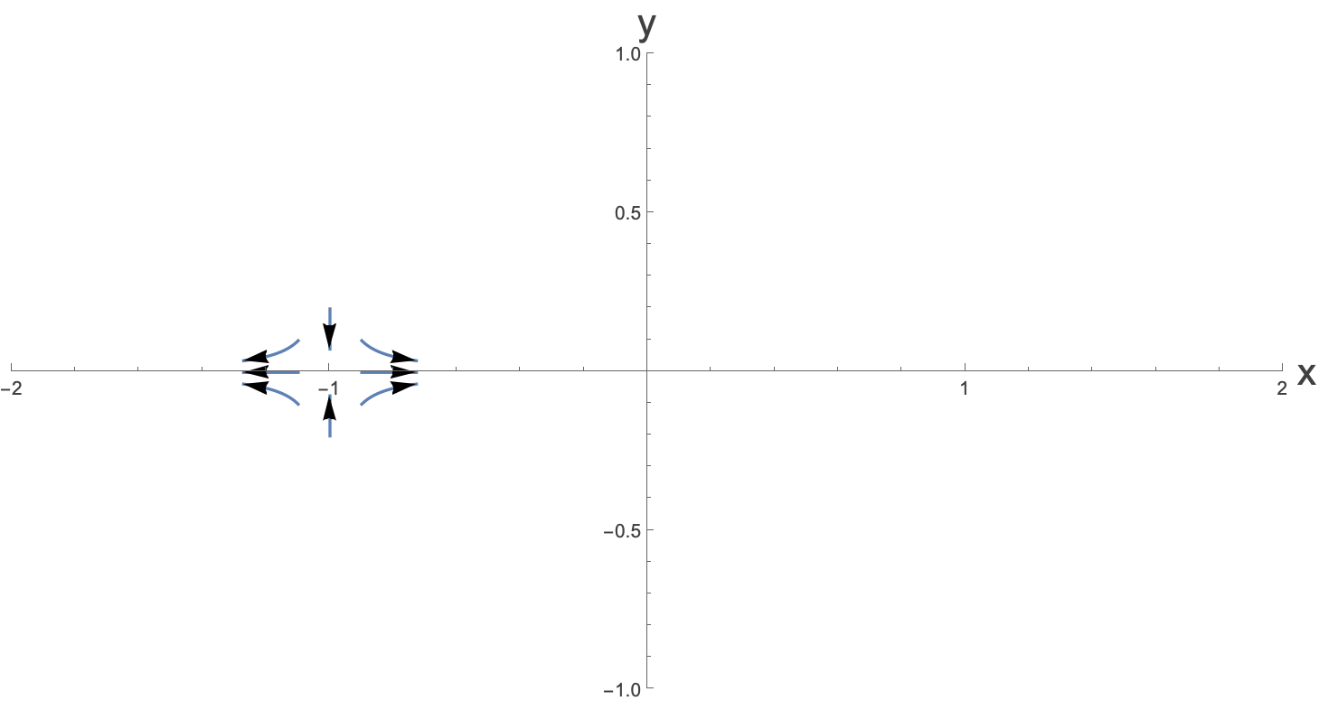
If we plot this vector field close to the fixed point we see:

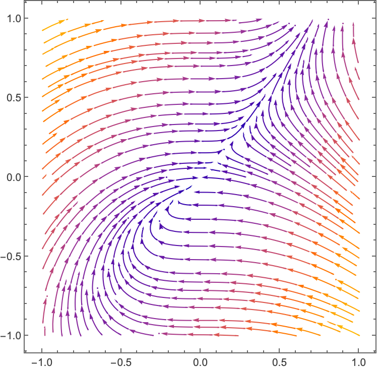
Where the fixed point at the center simply isn’t one of the linear fixed points, in any limit. It’s kind of saddle-pointesque…there are lines flowing in, and lines flowing out, but it ’s a pretty weird one.

We will talk more about these non-linearisable fixed points when we talk about index theorems.

Assignment

OK, now it’s your turn!

We’re going to look at a population of dassies (D, in units of 1000 dassies) and baboons (B, in units of 1000 baboons). Both of them feed on the same plants in the same area, so they are competing for resources. If we only had baboons, or only dassies, then the population could be modelled by the logistic equation. There would be some carrying capacity meaning that the environment could only sustain a certain sized population. Things change a bit when they are both in the same environment and they are both in competition for the same resource. We can write down the following non-linear model for the two populations:

$$ \dot{B}=B\left(2-B-D\right) $$$$ \dot{D}=D\left(3-2B-D\right) $$

1. Explain why these equations seem reasonable. You don’t need to explain the numbers specifically, but give a general explanation for each term and the relative magnitude of the numbers.

2. Now calculate the fixed points of this system. There should be four of them. Plot them in the (B,D) plane.

3. For each fixed point, calculate the Jacobian and calculate Δ and τ. Locate these fixed points in the (Δ,τ) plane and discuss the nature of each fixed point.

4. Calculate the eigenvalues and eigenvectors associated to each fixed point.

5. Draw in arrows corresponding to the flows close to each fixed point.

6. Now draw in what you might guess to be the flows outside of the fixed point regions. Note that you are quite constrained by the fact that you know that flows cannot cross one another.

7. For a saddle-point, the incoming flows correspond to a stable manifold. Label this in the figure.

8. Interpret what this phase diagram is telling you about the ecological system.

9. Assuming that you don’t start off exactly at any of the fixed points, what are the possible long-term situations in this environment. Why do you think that this might be called The Principle of Competitive Exclusion?

10. Shade in the region in the plot from which you will end up with only dassies as $t\to \infty{}.$ This region is known as a Basin of Attraction for the point $\left(0,N_{D}\right)$ where $N_{D}$ is whatever the non-zero stable fixed point for dassies is. Note that the stable manifold separates the two basins of attraction in this model. The trajectories of the stable manifold are called the Separatrices.