Section 0.0: Course Introduction
Section 0.0: Course Introduction
If you find any mistakes, or have comments on the notes, please message me at jon.shock@gmail.com.
This is the second year course which follows the first year course, MAM1043H. Notes for MAM1043H can be found here. The next couple of paragraphs are the same as those in the previous course.
The textbook that I will be following is: Nonlinear Dynamics and Chaos, by Steven Strogatz.
You do not need to get it. I will aim for this all to be self-contained. However, it is a beautifully written book, and almost certainly the best introduction to the subject.
Steven Strogatz actually has some of the material that we will be covering on Youtube: here.
He has in the past tweeted to this link which has some Python code for some of the examples in the book.
Here are some more links to online courses which you may want to browse.
- Complexity Explorer course on intro to dynamical systems and chaos
- Complexity Explorer course on introduction to differential equations
Please note, that I will often put in links to Wikipedia articles. One has to be careful about how accurate Wikipedia pages are, and in general if you are writing a scientific research paper, Wikipedia articles are not good to reference. However, for an educational set of notes like this, where I think that it will add useful content, I will be doing so. Wikipedia articles should be read with a critical hat on, and if you want to dig further, look at the references in the articles themselves.
What is this course about?
- Understanding what a dynamical system is through examples and definitions
- Knowing how to write down the mathematics of a dynamical system through examples and problems
- Knowing how to understand the interactions of dynamical systems through quantitative and qualitative means through many different techniques
I am writing these notes using the Wolfram Mathematica programming language. It means that I can very easily include nice plots and animations which should add to the content. You do not need to know how to use this.
The Course Content:
Section 1: Two dimensional nonlinear systems (Strogatz chapter 6)
- 1.1 Phase portraits in two dimensions
- 1.2 Existence and uniqueness
- 1.3 Fixed points and linearisation
- 1.4 Conservative systems
- 1.5 Reversible systems
- 1.6 Index theory
Section 2: Limit cycles (Strogatz chapter 7)
- 2.1 Limit cycles
- 2.2 Ruling out closed orbits
- 2.3 The Poincare-Bendixson theorem
- 2.4 Lienard systems
- 2.5 Relaxation oscillations
- 2.6 Weakly nonlinear oscillators
Section 3: Bifurcations (Strogatz chapter 8)
- 3.1 Saddle-nodes, transcritical and pitchfork bifurcations
- 3.2 Hopf bifurcations
- 3.3 Oscillating chemical reactions
- 3.4 Global bifurcations of cycles
- 3.5 Coupled oscillators and quasiperiodicity
- 3.6 Poincare maps
Section 4: Chaos (Strogatz chapter 9)
Chapter 0: Reminder
The scientific method often goes something like this:
- Find some phenomenon that you want to understand.
- See if you can translate that phenomenon into the language of mathematics.
- Study the mathematics to see if you can make predictions.
- Test those predictions in the real world.
- If the predictions turn out to be true, make some more until you break your model.
- When the predictions turn out not to be true, change your model until it matches the world.
This way you are slowly but surely moving towards a more and more accurate picture of the world. There are a number of disclaimers to all of this. One is that you don’t want to keep making your model of the world more and more complicated (see the epicyclic model of the solar system). You want it to be as simple as possible while capturing everything that you observe - ie. as simple as possible, but no simpler. You may ask why we want to break your model. Well, this is due to the statement at the beginning of this chapter from George Box. If we want to find out where our model is wrong, the best way to do this is to find out where it breaks.
The models of the world that we will be interested in in this course are those can be expressed in terms of differential, or difference equations. In fact, this captures a small proportion of all accessible phenomena. Sometimes the language might be in terms of integro-differential equations, and sometimes one will want to use methods in combinatorics, differential geometry, topology, etc. to understand them, but in this course we will be using perhaps a little topology, but mostly relatively simple mathematics to understand the general behaviours of systems of non-linear differential equations, generally of 2 or 3 coupled variables.
When we are talking about differential equations, we can completely generally write down a first order coupled system of two variables as follows:
$$ x'\left(t\right)=f\left(x\left(t\right),y\left(t\right)\right) $$$$ y'\left(t\right)=g\left(x\left(t\right),y\left(t\right)\right) $$where $f$ and $g$ are some specified functions of $x$ and $y$.
We started off last year talking about differential equations where we had a single function, of the form:
$$ x'\left(t\right)=f\left(x\left(t\right)\right) $$and we found that there was some interesting phenomena to discover even in this very simple setting. However, there were a number of things which we proved could not happen, for instance you can’t have oscillations in a one dimensional system (remembering that if we add in time dependence this is equivalent to looking at a two dimensional system).
In the last part of MAM1043H we looked at two dimensional systems, but ones where $f$ and $g$ were linear functions. This allowed us to write the equation as a matrix equation of the form.
$$ x'\left(t\right)=A x\left(t\right) $$Where
$$ x=\left(\begin{matrix} x \\ y \end{matrix}\right) , A=\left(\begin{matrix} a & b \\ c & d \end{matrix}\right) $$We are actually going to be able to use lots of the machinery that we developed in the first year, so remind yourselves of this here. There is also a very nice set of lecture notes which gives a detailed overview of such systems. I’d definitely recommend using this as a resource.
The main thing to remember about this is that to find the different types of behaviour, you need to calculate the determinant (Δ) and trace (τ) of the matrix $A$. We could then plot the different types of behaviour in a two dimensional space like this:
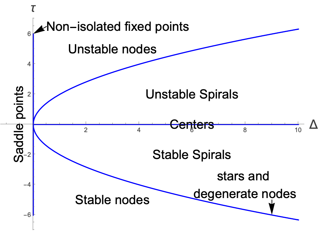
This plot alone will help us a lot when we move on in the next section to the non-linear case.